
Recursion-transform method and potential formulae of the m×n cobweb and fan networks∗
2017-08-30 08:25ZhiZhongTan谭志中
Chinese Physics B 2017年9期
Zhi-Zhong Tan(谭志中)
Department of Physics,Nantong University,Nantong 226019,China
Recursion-transform method and potential formulae of the m×n cobweb and fan networks∗
Zhi-Zhong Tan(谭志中)†
Department of Physics,Nantong University,Nantong 226019,China
In this paper,we made a new breakthrough,which proposes a new recursion–transform(RT)method with potential parameters to evaluate the nodal potential in arbitrary resistor networks.For the first time,we found the exact potential formulae of arbitrary m×n cobweb and fan networks by the RT method,and the potential formulae of infinite and semi-infinite networks are derived.As applications,a series of interesting corollaries of potential formulae are given by using the general formula,the equivalent resistance formula is deduced by using the potential formula,and we find a new trigonometric identity by comparing two equivalence results with different forms.
recursion-transform method,network model,potential formula,exact solution
1.Introduction
Searching for potential formula and equivalent resistance formula of resistor networks is a classic research topic in electric circuit theory and physics.An important development in circuit theory is that Kirchhoff,a German scientist,established the node current law and the circuit voltage law in 1845.[1]From then on,resistor network models have been researched more than 170 years.Nowadays,the resistor networks are attracting more and more attention because they can be used in both electrical and non-electrical system models,and the simulation through modeling resistor networks has become a basic method to solve complicated problems in the fields of engineering and science.[1–43]For example,the computation of resistance is relevant to problems ranging from classical transport in disordered media,[2]electro migration phenomena in metallic lines,[3]first-passage processes,[4]lattice Greens functions,[5]random walks[6]to hybrid graph theory.[7]Modeling resistor networks are also useful for researching exactfinite-size corrections in critical systems.[8,9]In addition,in physics and probability theory,the mean field theory can be used to study the behavior of large and complex stochastic models by studying simpler models such as finite disordered networks.[10–12]The mean field theory has also been widely used in statistical mechanics,condensed matter in complex systems,magnetism,structure transition,and other fields.In order to obtain an analytical solution,the resistance of a regular resistor network with a perfectly ordered structure is calculated.If the heterogeneity is weak,the mean-field approximation is valid.[10–12]
The potential theory is an important theory in natural science and engineering,for example,Laplace equation is a kind of second-order partial differential equation,Poisson equation is a kind of inhomogeneous Laplace equation,[13–19]and Laplace equation and Poisson equation are the simplest examples of elliptic partial differential equations.The general theory of solutions to Laplace equation is known as the potential theory.The solutions of Laplace equation,which are all harmonic functions,are important in many fields of science and engineering,notably in electromagnetism,astronomy,and fluid dynamics,as they can accurately describe the behaviors of electric,gravitational,and fluid potentials.In heat conduction study,the Laplace equation is the steady-state heat equation.The potential function has been applied not only in the electrical theory,but also in non-electric fields,such as potential fields obeying Laplace equation,although the physical properties of different potential fields are different but if they have similar boundary conditions.Due to the uniqueness of Laplace equation,a potential field of solution or the potential field model experiment of surveying and mapping of hot surface or flow chart can be shared with other potential fields after corresponding physical quantity of conversion.Thus, a large number of studies in natural science and engineering can be solved by the potential function equation.However, problems in real life are usually complicated because of different boundary conditions.A tiny change of boundary conditions affects the solutions.Therefore,accurately calculating the solution of Laplace equation under complex boundary conditions is difficult and approximate methods are usually used to obtain approximation solutions which meet actual needs,in which a common method called the finite difference methodwas established to study the approximate solutions of differential equations and integral differential equations.[13–19]The basic idea of the finite difference method is to use a finite number of discrete points of grid instead of a continuous definite region,these discrete points are called grid nodes,and that is to say,the finite difference method is implemented by means of grid models.Because network models have specific visual features,if we use the resistor network model to solve the finite difference problem,the electric potential of each node will represent the solution of function equation to be solved.If the potential analytical solution of each node in the resistor network model is obtained,we can precisely obtain the analytical solution of differential equations.However,to find exact solutions of nodal potential in resistor networks is important but difficult,the previous theory has not been work out the precise formula of electric potential of each node in resistor network models.
From the research history,we find that it is difficult to obtain the exact potential and resistance in an arbitrary m×n resistor network with an arbitrary boundary,because the boundary is like a wall or trap which affects the behavior of finite networks.[20–36]Therefore,several different effective methods used to calculate the equivalent resistances of resistor networks with different geometric constructions have been proposed.In 2000,Cserti[20]evaluated the two-point resistance of infinite lattices by using Green function,which cannot be applied to finite resistor networks.In 2004,Wu[22]proposed a different approach(called Laplacian matrix method)and derived explicit expressions of two-point resistance in arbitrary finite and infinite lattices in terms of the eigenvalues and eigenvectors of the Laplacian matrix relying on two matrices along two vertical directions.After that,the Laplacian approach has been extended to complex impedance networks[23]and resistor networks with a zero resistor boundary.[24,25]However,as the Laplacian method cannot be applied to a matrix with arbitrary elements,which is incapable to solve the eigenvalue problem, this approach cannot solve resistor network problems with arbitrary boundaries.
In recent years,a new recursion transform(RT)method was proposed by Tan,[26–28]the RT method,depending on one matrix along one direction,is different from the Laplacian method.With the development of RT technique,some problems of resistor networks have been resolved.[26–36]Although fruitful research results on the equivalent resistance of resistor networks have been obtained,the nodal potential of the resistor network has not been obtained.Therefore,in this paper,we make a new breakthrough for studying the nodal potential of resistor networks.The previous RT method[26–28]is based on current parameters,this paper further generalizes the RT method and promotes the RT method to suit to potential parameters.We find that the RT method can solve the analytical solutions of the potential of each node in resistor network models,thus our method can solve the Laplace equation with complex boundary conditions.
In addition,the resistor network model,which has been applied to a number of disciplines,is an interdisciplinary subject.[37–43]Therefore,the construction of and research on resistor network models can be useful in theory and application.
In this paper,we investigate the potential formula of arbitrary m×n cobweb and fan networks,which have not been resolved before.We focus on providing a new theory and technique useful for related scientific research.
This paper is organized as follows.In Section 2,we present potential formulae of the cobweb and fan resistor networks.In Section 3,we illustrate RT method by using the cobweb network model.In Section 4,some new applications of potential formulae in infinite and semi-infinite cases are given. Section 5 gives the discussion and summary.
2.The main result:potential formula
2.1.Potential formula of the cobweb network
We consider an arbitrary m×n resistor cobweb network with resistors r0and r in the respective longitude(radius)and latitude(circle)directions,where m and n are,respectively,the numbers of resistors along longitude and latitude directions as shown in Fig.1.Assume that the center node O is the origin of the rectangular coordinate system and a longitude acts as Y axis.Denote the nodes of the network by coordinate{x,y} and the potential of node d(x,y)is Um×n(x,y)=V(y)xas shown in Fig.2.
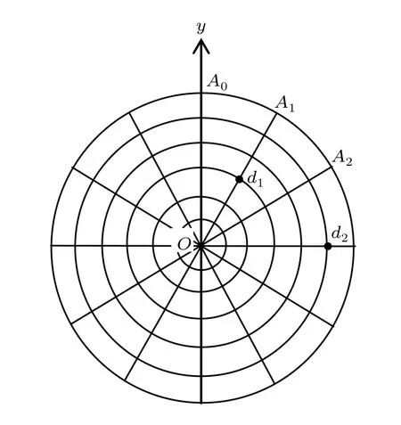
Fig.1.An 6×12 resistor cobweb network,where 6 and 12 are,respectively,the numbers of resistors along longitude and latitude directions.
By assuming that the current J goes from d1(x1,y1)to d2(x2,y2),selecting d0(0,0)as the reference point of the potential,and Um×n(0,0)=0,the potential of an arbitrary node in the m×n cobweb network can be written as
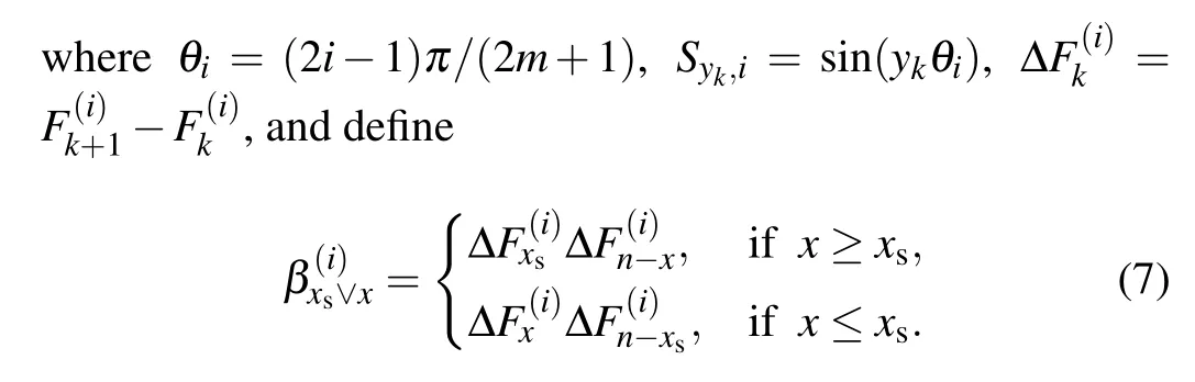
where θi=(2i−1)π/(2m+1),Syk,i=sin(ykθi),and
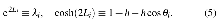
Define h=r/r0and
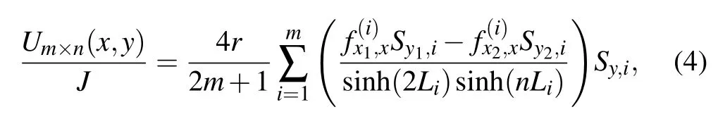
In addition,equation(1)can be expressed in another form as
2.2.Potential formula of the fan network
Consider an arbitrary m×n resistor fan network with resistors r0and r in the respective longitude and latitude directions,where m and n are,respectively,the numbers of resistors in longitude and latitude directions as shown in Fig.3. All definitions of parameters are the same as these in the section above.The potential of an arbitrary node in the m×n fan network can be written as
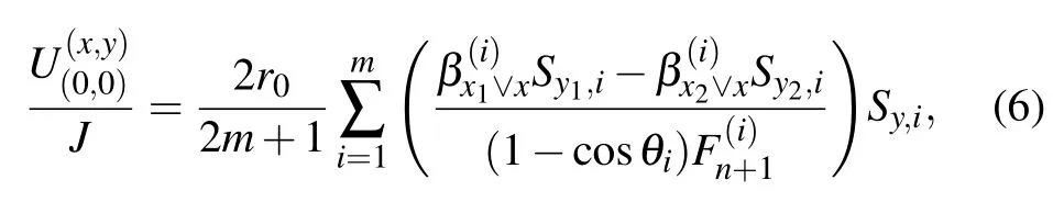
In particular,when the output current J is at the center of O(0,0)(the origin of coordinates)and the input current J is at the left edge of d1(0,y1),the potential formula of the node d(x,y)in the m×n fan network can be written as
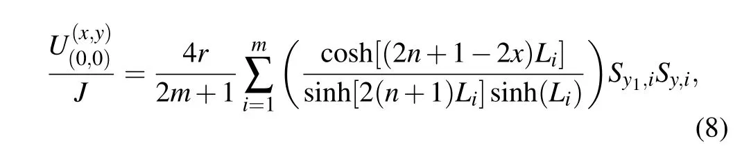
where θi=(2i−1)π/(2m+1)and Lihas been defined in Eq.(5).
Equations(1),(4),(6),and(8)are potential formulae of point d(x,y)in arbitrary m×n cobweb and fan resistor networks,which are found for the first time.In the following sections,we derive them by using the RT method with potential parameters.
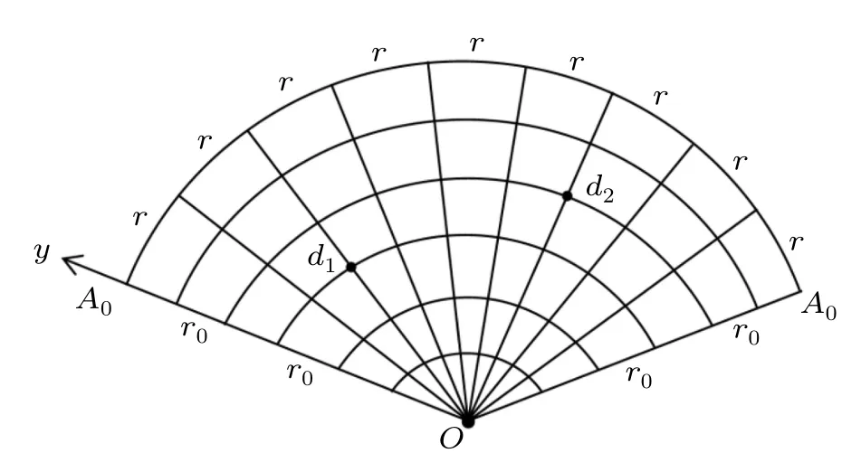
Fig.3.A fan m×n resistor network,where m and n are,respectively, the numbers of resistors along longitude and latitude directions.
3.A general theory and approach
In this section,we first derive Eqs.(1)and(4),and then derive Eqs.(6)and(8)by the generalized RT method.The RT method divides the derivation into four steps:first,construct a matrix relation between the potentials in three successive transverse lines;second,derive a recursion relation between the potentials on the boundary;third,diagonalize the matrix relation to produce a recurrence relation involving only variables in the same transverse line;fourth,implement the inverse transformation of matrix to yield the node potential.
3.1.Modeling the matrix equation
Consider that the center node O is the origin of the rectangular coordinate system and longitude OA0acts as Y axis as shown in Fig.1.Denote the nodes of the network by coordinate{x,y},denote the potential in all segments of the network as shown in Fig.3,and assume that the potentials at node d(x,y)isand at the center is.
Firstly,we research the segment of resistor networks with potential parameters as shown in Fig.3.We focus on four rectangular meshes and nine nodes,using Kirchhoff’s current lawto the node along the longitude axis of k th,we can obtain the node potential formula as follows by ignoring the external current source:
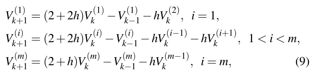
where h=r/r0.Equation(9)can be written in an matrix form by considering the injection of J at d1(x1,y1)and the exit of J at d2(x2,y2),
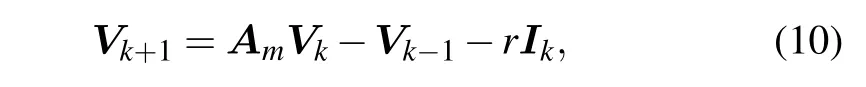
where Vkand Ikare,respectively,m×1 column matrices,and reads
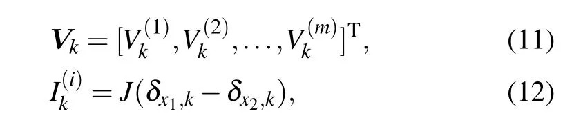
where[]Tdenotes matrix transpose and
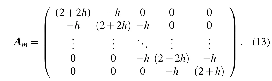
Second,we consider the boundary conditions in Y axis of the network.Applying Kirchhoff’s current lawto the nodes adjacent to Y axis,we obtain
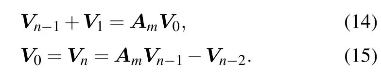
where matrix Amhas been given in Eq.(13).
Equations(10)–(15)are all equations needed to calculate the potential formula.However,it is impossible for us to obtain the solution of the potential matrix directly by Eqs.(10)–(15).How to solve matrix equation(10)is the key to the problem.Therefore,we establish the following method of matrix transform to resolve this problem indirectly,the matrix transform method is our key technique.
3.2.Approach of matrix transform
Because equation(10)is a complex matrix equation whose solution cannot been obtianed directly,we rebuild a new difference equation and solve Eq.(10)indirectly by means of matrix transform in this subsection.
Firstly,we multiply Eq.(10)at the left side by an m×m undetermined square matrix Pm,

Construct the transformation of diagonal matrix by the following two identities:
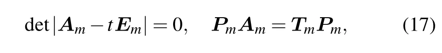
where Emis an m×m identity matrix and Tm= diag(t1,t2,...,tm).Since Amis a special tridiagonal matrix which is Hermitian,it can be diagonalized by a similarity transformation.Solving Eq.(17),we obtain
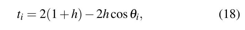
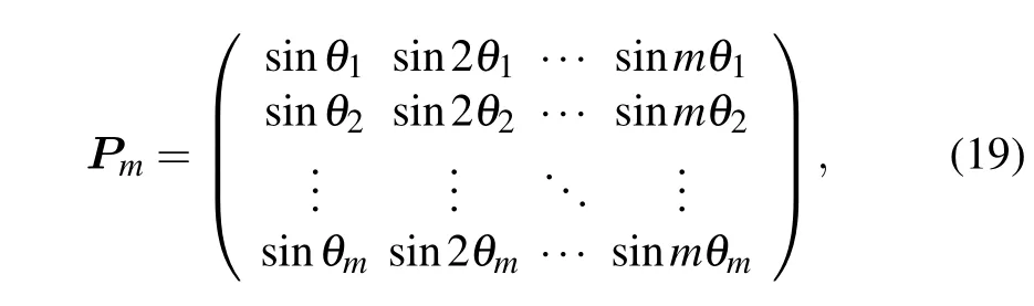
where θi=(2i−1)π/(2m+1)and the matrix of eigenvectors is(one may refer to Ref.[32])
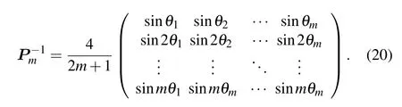
with the inverse matrix(one may refer to Ref.[32])
For convenience,by Eqs.(16)and(17),letting
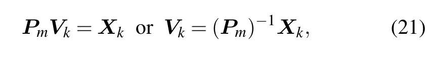
where Xmis an m×1 column matrix and reading
thus,we obtain the following main equation after applying Eqs.(17)and(21)to Eq.(16):

where(simply read ζy1,ias ζ1,i,and ζy2,ias ζ2,i)

We conduct the same matrix transform as used in Eq.(23).Applying Pmto Eqs.(14)and(15)on the left-hand side,we obtain
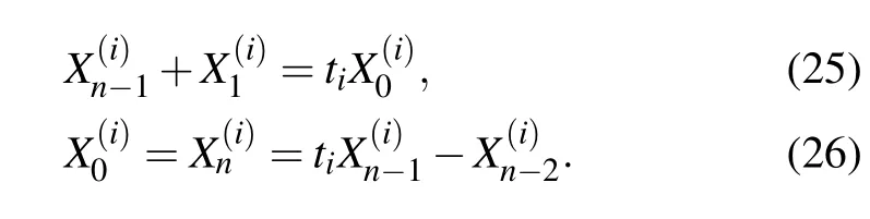
Equations(23)–(26)are all essential equations for solving the potential by solving the matrix ofBy using the above matrix transform,we can obtain variablewith potential parameters.
3.3.General solutions of the matrix equations
Next,we derive the exact solution of Xkby Eqs.(23)–(26).Supposing that λiandare the roots of the characteristic equation for Xkin Eq.(23),we obtain the characteristic roots(3)according to Eq.(23).
From Eq.(23),we obtain the piecewise solutions after considering the injection of current J at d1(x1,y1)and the exit of current J at d2(x2,y2),
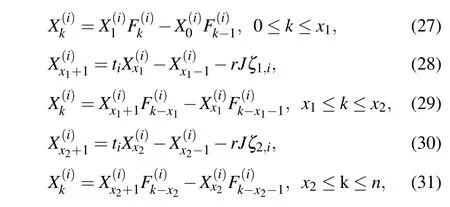
Solving matrix equations(25)–(31),we obtain the general solution ofwith potential parameters(0≤k≤n),
where ζ1,iand ζ2,ihave been given in Eq.(24)andhas been defined in Eq.(2).
3.4.Matrix inverse transform
In this section,we derive the potential formula by matrix inverse transformation.Using Eq.(21),Vk=(Pm)−1Xk,and expanding the inverse matrix,we have
According to Eq.(33),we have
Substituting Eq.(24)into Eq.(35),we therefore obtain Eq.(1).
In addition,when λi=e2Li(one may refer to Ref.[30]), substituting toyields
Since λi=e2Liand=e−2Li,we have
Substituting Eqs.(36)–(38)into Eq.(1),we therefore obtain Eq.(4).
3.5.Deriving quations of the fan network
Similar to that of the cobweb network,we calculate the potential of fan network by an major matrix equation and two boundary condition equations.The major matrix equation of the fan network is just exactly the same as Eqs.(9)–(13), and its main transformation matrix is just Eq.(23),while the boundary condition equations of the fan network are different from those of the cobweb network,they are
We conduct the same matrix transformation as that in Eq.(16). Applying Pmto Eqs.(39)and(40)on the left-hand side,we obtain
Equations(23),(41),and(42)are all essential equations for solving the potential of the fan network.Similar to the derivation of the cobweb network,by Eqs.(23),(41),and(42), we work out after some algebra and reduction the general solution ofwith potential parameters(0≤k≤n),
where tihas been given in Eq.(18)andhas been defined in Eq.(7).
Next,we derive the potential formula by matrix inverse transformation.Using Eq.(21),we have Vk=(Pm)−1Xk,together with Eqs.(20)and(43),we therefore obtain

Substituting Eq.(24)into Eq.(44),we therefore obtain Eq.(6).
In addition,similar to the approach to prove Eq.(4),we can easy prove Eq.(8)by using
For the first time,we obtained two general potential formulae of arbitrary m×n cobweb and fan networks by the RT method,which provides a new theoretical method for related scientific research.
4.Applications of the potential formula
In this section,we mainly give a series of specific applications of the potential formula of the cobweb network under different conditions.In the applications below,we always assume thatand U(∞,∞)=0.
4.1.Specific potential in the finite network
Application 1 Consider an arbitrary m×n cobweb resistor network as shown in Fig.1.Assume that the output current J locates at the center of O(0,0)(the origin of coordinates), the input current J locates at an arbitrary node d1(x1,y1),the potential formula of the node d(x,y)in an arbitrary m×n cobweb network can be written as
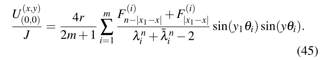
Derivation of Eq.(45)is as follows.
When the output current locates at the center of O(0,0), y2=0 and the input current locates at the node of d1(x1,y1), we obtain
Substituting Eq.(46)into Eq.(1),we immediately obtain Eq.(45).
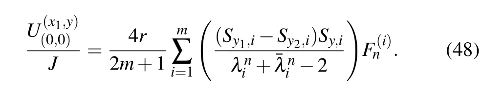
Application 2 When the input current and output current locate in the same longitude,the current J goes from node d1(x1,y1)to node d2(x1,y2).From Eq.(1)with x2=x1,the potential formula of node d(x,y)in the m×n cobweb network can be written as
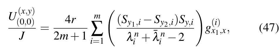
In particular,when the node d(x,y)=d(x1,y)locates in the same longitude axis with d1=(x1,y1)and d2=(x1,y2), the potential formula(47)reduces to
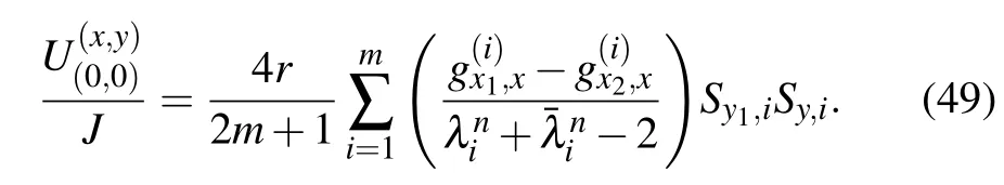
Application 3 When the current J goes from d1(x1,y1)to d2(x2,y1)and the two current nodes locate in the same latitude, from Eq.(1)with y2=y1,the potential formula of an arbitrary node d(x,y)in the m×n cobweb network can be written as
Application 4 In Fig.1,assume that the current J goes from d1(x1,y1)to the two output nodes of d2(x2,y2)and d3(x2,y3),where two output currents are respectively J/2,this situation is regarded as two independent current sources.From Eq.(1),the potential formula of an arbitrary node d(x,y)in the m×n cobweb network can be written as
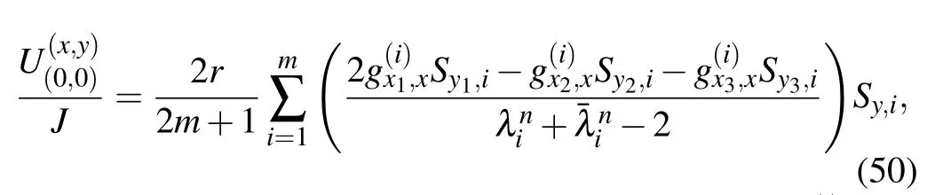
where Sk,i=sin(ykθi)has been given in Eq.(1)andhas been defined in Eq.(2).
Application 5 When the input current has k nodes,assume that the output current J locates at the center node O(0,0)and the input currents have k nodes of dk(xk,y1)(k= 1,2,...,k)in the same latitude,which is J/k.The potential at node d(x,y)is composed of the sum of k potentials.From Eq.(45),we have the potential formula
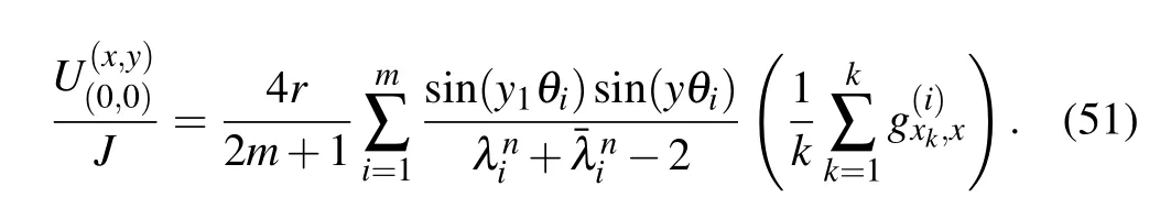
Application 6 When the input current has n nodes,assume that the output current J locates at the center node O(0,0)and the current inputting to node dk(xk,y1)(k= 1,2,...,n)in the same latitude is J/n.From Eq.(51),we have the potential formula
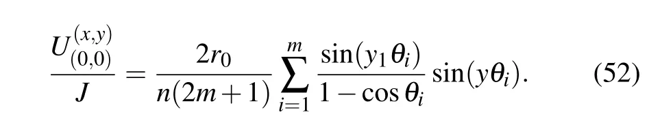
Derivation of Eq.(52)is as follows.
When there are n independent current sources,each node potential is the summations of n potentials since the potential is a scalar.Using Eq.(51)with k=n,we compute the sums ofFrom Eq.(2),we have

Substituting Eq.(53)into Eq.(51)with k=n,we therefore obtain Eq.(52).
Equation(52)gives an interesting result as it has nothing to do with x,but only related to y.This equation shows that the nodes in the same latitude have the same potential,which is completely in line with the facts.
4.2.The potential in the infinite network
Application 7 Assume that figure 1 shows an infinite network and the electric current J goes from node d1(x1,y1)to node d2(x2,y2).By supposing the potential at node d0(0,0)is U(0,0)=U(∞)=0,the potential formula of node d(x,y)can be written as
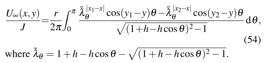
Derivation of Eq.(54)is as follows.
In order to derive Eq.(54),the following integral theory is necessary.If φk=(2k−1)π/(2m+1),we have Δφk= φk+1−φk=2π/(2m+1).In the limit of m→∞,we have
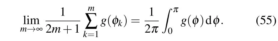
First,we consider the case of n→∞with finite m.By using Eq.(2),we obtain

Taking m,n→∞and applying Eqs.(55)and(56)to Eq.(1), we therefore obtain Eq.(54).
4.3.Expressing the potential by resistance
Application 8 Assume that figure 1 shows an infinite network and the electric current J goes from node d1(x1,y1)to node d2(x2,y2).By supposing U(0,0)=U(∞)=0,the potential formula of node d(x,y)can be written as
where Rddkrepresents the resistance between two nodes d(x,y) and dk(xk,yk)in an infinite network,which is(one may refer to Ref.[27])
4.4.The potential formula in the semi-infinite network
Application 9 Assume that figure 1 shows a semi-infinite cobweb network,where m is infinite,but the grid number n in the latitude line is finite,and(x,y)and(x1,y1)are finite. When the output current is at node O(0,0)and the input current is at node d1(x1,y1),the potential of node d(x,y)in the semi-infinite cobweb network can be written as
In particular,when m,n→∞,y1,y and x1−x are finite, taking n→∞in Eq.(59),we obtain the potential of node d(x,y)in the semi-infinite cobweb network as
4.5.Application of the potential of an infinite network
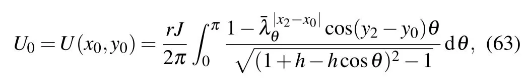
Application 10 Assume that figure 1 shows an infinite network,the input current J locates at d0(x0,y0),and the output current locates at infinity.By supposing that the potential at node d0(x0,y0)is U0,the node potential of an infinite cobweb network can be written as
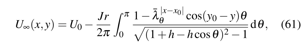
Derivation of Eq.(61)is as follows.
Assuming that the input current J locates at d0(x0,y0)= d1(x1,y1),from Eq.(54),we have
and then,the potential difference between two nodes d(x,y) and d0(x0,y0)is
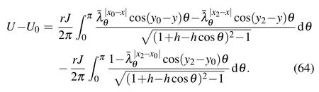
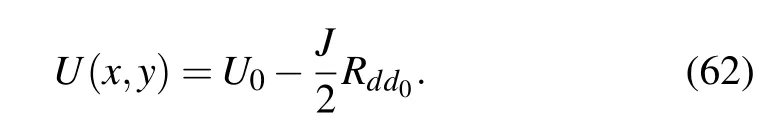
Since d2(x2,y2)locates at infinity,then x2,y2→∞,becauseand x is finite,we have0,thus,taking Eq.(64)to limit,we therefore obtain Eq.(61). In addition,applying Eq.(58)to Eq.(61),we immediately obtain Eq.(62).Please note that equations(61)and(62)are only suitable when the output current is at infinity.
Application 11 Assume that figure 1 shows an infinite network,the input and output currents locate in the same latitude,and the current J goes from d1(x1,y1)to d2(x2,y1),suggest the potential at infinity is zero.According to Eq.(54),the potential of node d(x,y)can be written as
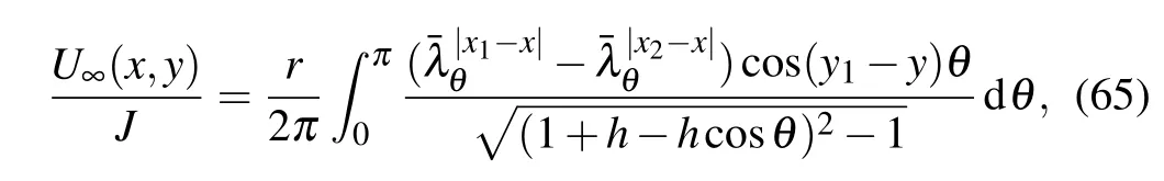
The coordinate scope of Eq.(65)is suitable for all coordinates.
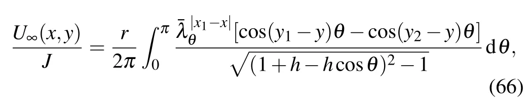
Application 12 Assume that figure 1 shows an infinite network,the input and output currents locate in the same longitude,and the current J goes from d1(x1,y1)to d2(x1,y2). Suppose the potential at infinity is zero.According to Eq.(54) the potential of node d(x,y)can be written as
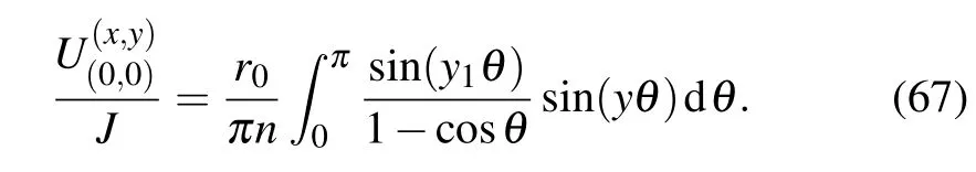
Application 13 Consider a semi-infinite∞×n cobweb network,assume that the output current at the center node O(0,0)is J and the current input to the nodes dk(xk,y1)(k= 1,2,...,n)in the same latitude is J/n.Applying Eq.(55)to Eq.(52),we obtain the potential formula of the semi-infinite network
As we all know,it is difficult to compute the potential based on the multiple nodes of the current input and current output in science.However,the research methods in this paper can resolve this problem.
4.6.Resistance formula of an m×n cobweb network
Application 14 Consider an arbitrary m×n resistor cobweb network with resistors r and r0in the respective latitude and longitude,where m and n are,respectively,the numbers of grids along longitude and latitude directions as shown in Fig.1.The equivalent resistance between two arbitrary nodes d1(x1,y1)and d2(x2,y2)in an arbitrary m×n cobweb network can be written as
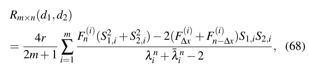
where Δx=|x2−x1|,Sk,i=sin(ykθi),andand λihave been,respectively,defined in Eqs.(2)and(3).
The derivation of Eq.(68)is as follows.
Suggesting that the potentials at nodes of d1(x1,y1)andand by Ohm’s law,we have
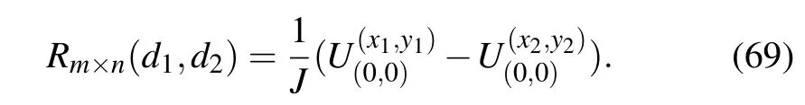
Substituting(x,y)=(x1,y1)and(x,y)=(x2,y2)into Eq.(1), we obtain the values ofsubstituting them into Eq.(69),we therefore obtain Eq.(68).
Application 15 Similar to the derivation of Eq.(68),using Eq.(4),we obtain another resistance formula expressed by the hyperbolic functions as

where Li=lnλi/2,Sk,i=sin(ykθi),Δx=|x2−x1|,and λihas been defined in Eq.(3).
Please note that the resistance of an arbitrary m×n resistor cobweb network has been studied in Refs.[24],[28], and[31],by comparison,we find that all resistance equatons are completely equivalent although different calculation methods were used.
4.7.Resistance formula of an m×n fan network
Application 16 Consider an arbitrary m×n resistor fan network with resistors r and r0in the respective latitudes and longitudes,where m and n are,respectively,the numbers of grids along longitude and latitude directions as shown in Fig.2.Assume that the center node O is the origin of the rectangular coordinate system and the left edge acts as Y axis. Denote nodes of the network by coordinate{x,y}.The equivalent resistance between two arbitrary nodes d1(x1,y1)and d2(x2,y2)in an arbitrary m×n fan network can be written as
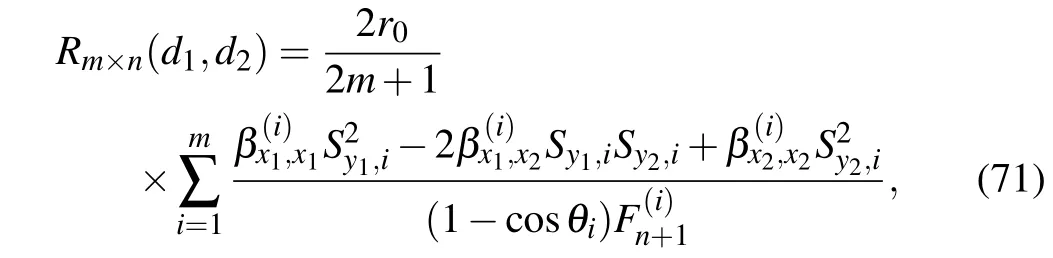
In particular,when d1(x1,y1)=(0,0)is at the center O, from Eq.(71),we have the resistance formula
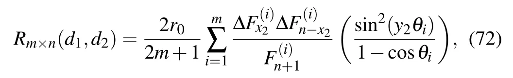
Please note that the resistance of an arbitrary m×n resistor fan network has been researched in Refs.[27]and[31], by comparison,we find that all resistance formulae are completely equivalent although different calculation methods were used.
4.8.Comparation and product identities
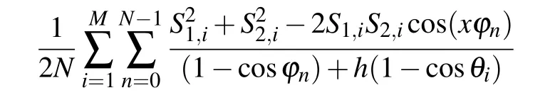
Reference[24]gave a resistance formula between two arbitrary nodes in m×n cobweb resistor networks by means of the Laplacian matrix method,which is in the form of double sums.The equation is

where x=x2−x1,Sk,m=sin(ykθm)and ϕn=2nπ/N,θm= (2m−1)π/(2M+1).
This paper gives Eq.(68)by the RT method,obviously, the two results with different forms are necessarily equivalence because they are from the same network with the same coordinates.Comparing Eq.(68)with Eq.(73),we immediately obtain a new identity below.
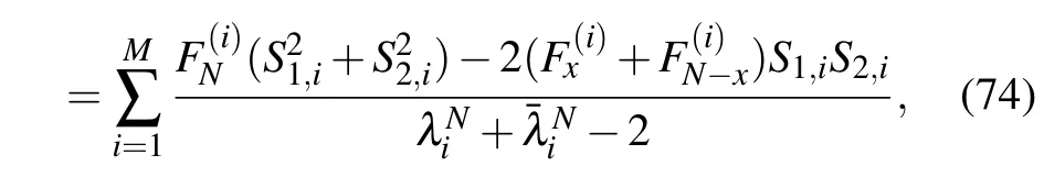
where λiandhave been given in Eq.(3).
Equation(74)is interesting as it simplifies double sums to a single sum.In particular,when x,m,n and y1,y2are specific values,we have the following simple trigonometric identities.
Case 1 When y1=y2,equation(74)reduces to
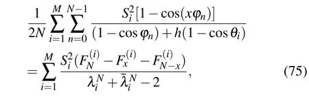
where Si=sin(y1θi),θi=(2i−1)π/(2M+1),and ϕn= 2nπ/N.
Case 2 When M=1,ϕn=2nπ/N,equation(74)reduces to
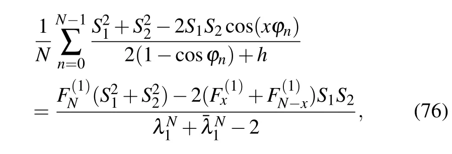
where S1=sin(y1π/3),S2=sin(y2π/3),y1={0,1},y2= {0,1},and
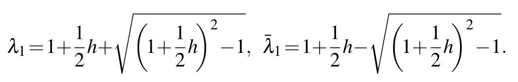
These identities are interesting because they come from physics rather than mathematics.Please note that the above identities are found for the first time by this paper.
5.Discussion and summary
In this paper,we obtained a series of exact potential formulae in arbitrary m×n cobweb and fan networks by developing the RT method.In some extent,we obtained the analytical solutions of Laplace equations in a variety of boundary conditions by the RT method,because Laplace equation can be simulated by resistor network models.
Take the cobweb network as an example,the RT method divides the derivation into four steps:first,construct the matrix relation of the currents(or voltages)in three successive transverse lines;second,build boundary condition equations of the currents(or voltages);third,diagonalize the matrix relation to produce a recurrence relation involving only variables in the same transverse line.Basically,the method reduces the problem from two dimensions to one dimension;fourth,implement the inverse transformation to matrix to calculate the node potential(or branch currents).
As applications,we obtained general potential formulae(1),(4),(6),and(8)in arbitrary m×n cobweb and fan resistor networks.The equivalent resistance formulae were deduced by using potential formulae(68),(70),and(72).As applications of Eq.(1),some interesting results were produced, and the resistance formulae(68),(70),and(72)were produced.The RT method and potential formulae(1),(4),(6), and(8)are useful in theory and practical applications.
[1]Kirchhoff G 1847 Ann.Phys.Chem.148 497
[2]Kirkpatrick S 1973 Rev.Mod.Phys.45 574
[3]Pennetta C,Alfinito E,Reggiani L,Fantini F,DeMunari I and Scorzoni A 2004 Phys.Rev.B 70 174305
[4]Redner S 2001 A Guide to First-Passage Processes(Cambridge:Cambridge University Press)
[5]Katsura S and Inawashiro S 1971 J.Math.Phys.12 1622
[6]Doyle P G and Snell J L 1984 Random Walks and Electrical Networks, The Mathematical Association of America,Washington,DC
[7]Novak L and Gibbons A 2009 Hybrid Graph Theory and Network Analysis(Cambridge:Cambridge University Press)
[8]Goodrich C P,Liu A J and Nagel S R 2012 Phys.Rev.Lett.109 095704
[9]Izmailian N S,Priezzhev V B,Philippe R and Hu C K 2005 Phys.Rev. Lett.95 260602
[10]Dobrosavljević V and Kotliar G 1997 Phys.Rev.Lett.78 3943
[11]Vollhardt D,Byczuk K and Kollar M 2011 Springer Series in Solid-State Sciences 171 203
[12]Caracciolo R,De Pace A,Feshbach H and Molinari A 1998 Ann.Phys. 262 105
[13]Weinan E and Wang X P 2000 SIAM J.Numer.Sci.Comp.38 1647
[14]Garcia-Cervera C J,Gimbutas Z and E W 2003 J.Comput.Phys.184 37
[15]Lai M C and Wang W C 2002 Numer.Methods Partial Differ.Equ.18 56
[16]Fornberg B 1996 A Practical Guide to Pseudo Spectral Methods(Cambridge:Cambridge University Press)p.17
[17]Houstis E,Lynch R and Rice J 1978 J.Comput.Phys.27 323
[18]Borges L and Daripa P 2001 J.Comput.Phys.169 151
[19]Kamrin K and Koval G 2012 Phys.Rev.Lett.108 178301
[20]Cserti J 2000 Am.J.Phys.68 896
[21]Giordano S 2005 Int.J.Circ.Theor.Appl.33 519
[22]Wu F Y 2004 J.Phys.A:Math.Gen.37 6653
[23]Tzeng W J and Wu F Y 2006 J.Phys.A:Math.Gen.39 8579
[24]Izmailian N S and Kenna R and Wu F Y 2014 J.Phys.A:Math.Theor. 47 035003
[25]Izmailian N S and Kenna R 2014 J.Stat.Mech.E 09 1742
[26]Tan Z Z 2015 Chin.Phys.B 24 020503
[27]Tan Z Z 2015 Phys.Rev.E 91 052122
[28]Tan Z Z 2015 Sci.Rep.5 11266
[29]Tan Z Z,Zhou L and Yang J H 2013 J.Phys.A:Math.Theor.46 195202
[30]Tan Z Z,Essam J W and Wu F Y 2014 Phys.Rev.E 90 012130
[31]Essam J W,Tan Z Z and Wu F Y 2014 Phys.Rev.E 90 032130
[32]Tan Z Z 2015 Int.J.Circ.Theor.Appl.43 1687
[33]Essam J W,Izmailian N S,Kenna R and Tan Z Z 2015 Roy.Soc.Open Sci.2 140420
[34]Tan Z Z 2016 Chin.Phys.B.25 050504
[35]Tan Z Z 2017 Commun.Theor.Phys.67 280
[36]Tan Z Z and Zhang Q H 2017 Acta Phys.Sin.66 070501(in Chinese)
[37]He Z W,Zhan M,Wang J X and Yao C G 2017 Fron.Phys.12 120701
[38]Tyson J J,Chen K and Novak B 2001 Nat.Rev.Mol.Cell Biol.2 908
[39]Xia Q Z Liu L L,Ye W M and Hu G 2011 New J.Phys.13 083002
[40]Davidich M I and Bornholdt S 2008 PLoS ONE 3 e1672
[41]Davidich M I and Bornholdt S 2013 PLoS ONE 8 e71786
[42]Bornholdt S and Rohlf T 2000 Phys.Rev.Lett.84 6114
[43]Davidich M and Bornholdt S 2008 J.Theor.Biol.255 269
14 May 2017;revised manuscript
7 June 2017;published online 2 August 2017)
10.1088/1674-1056/26/9/090503
∗Project supported by the Natural Science Foundation of Jiangsu Province,China(Grant No.BK20161278).
†Corresponding author.E-mail:tanz@ntu.edu.cn,tanzzh@163.com
©2017 Chinese Physical Society and IOP Publishing Ltd http://iopscience.iop.org/cpb http://cpb.iphy.ac.cn

- Chinese Physics B的其它文章
- Improved control for distributed parameter systems with time-dependent spatial domains utilizing mobile sensor actuator networks∗
- Geometry and thermodynamics of smeared Reissner–Nordström black holes in d-dimensional AdS spacetime
- Stochastic responses of tumor immune system with periodic treatment∗
- Invariants-based shortcuts for fast generating Greenberger-Horne-Zeilinger state among three superconducting qubits∗
- Cancelable remote quantum fingerprint templates protection scheme∗
- A high-fidelity memory scheme for quantum data buses∗