
Numerical solution of the Saint-Venant equations by an efficient hybrid finite volume/finite-difference method *
2018-05-14 01:42WencongLaiAbdulKhan
水动力学研究与进展 B辑 2018年2期
Wencong Lai, Abdul A. Khan
Glenn Department of Civil Engineering, Clemson University, Clemson, SC, USA
Introduction
Numerical modeling of overland flow and surface runoff, which is a major component of the water cycle, is of crucial importance in hydraulic and hydrologic engineering. For overland and open channel flows, 1-D, 2-D, or coupled 1-D and 2-D depth averaged shallow water flow equations are widely used for their simplicity and efficiency compared with the 3-D Navier-Stokes equations[1,2]. Numerical solutions of the hyperbolic shallow water flow equations(also called Saint-Venant equations) are computationally expensive and require a large computational effort. The challenges in numerical methods for the Saint-Venant equations include calculation of the numerical flux, treatment of source term, and simulating the wetting and drying processes[3,4]. Simplified and computationally efficient models such as the kinematic wave model[5,6], the diffusion wave model[7,8]and the inertial wave model[9,10]are often used in applicable flow conditions. These simplified models differ in physical propagation mechanism, computational complexity, and criteria of applicability[11-14].
The diffusion wave model and inertial wave model are good approximations to the dynamic wave model for flow with low Froude number[15,16]. Both the dynamic wave model and inertial wave model are based on hyperbolic equations, whose explicit solutions need to satisfy the linear relationship (between the maximum time step and the mesh size) governed by the Courant-Friedrichs-Lewy (CFL) condition. The diffusion wave model represents parabolic equations,where the maximum time step size in explicit schemes decreases quadratically with mesh refinements. Neal et al.[17]compared the performance of three 2-D explicit hydraulic models (dynamic, inertial, and diffusion models) in terms of efficiency and accuracy for flood inundation test cases. It was concluded that the diffusion wave model required the longest simulation times, while the inertial wave model required the shortest. The simpler models performed well in gradually varying flows, while the dynamic wave model is required to simulate super- critical flows accurately.
The Godunov-type finite volume method[18,19]and discontinuous Galerkin method[20,21]are suitable for numerical solutions of the Saint-Venant equations due to their conservation behavior and suitability for the hyperbolic system of equations. Computational efficiency of numerical solutions for the dynamic wave model is of interest and importance in practical use. The local time-stepping method[22], adaptive time-stepping method[23]and implicit time-stepping method[24]are proposed to increase run-time efficiency.
In this work, an efficient and accurate hybrid semi-implicit finite-difference and finite-volume method (SIFD-FVM) is developed to numerically solve the Saint-Venant equations. The finite-volume method is applied to the continuity equation, which results in a mass-conservative scheme. The finite volume method for the momentum equation can be complicated by the integral terms of pressure force and lateral force[25,26]and flux calculation[27,28]. A simple form of the momentum equation is solved using the semi-implicit finite-difference method without momentum flux calculation in order to achieve higher computational efficiency. An upwind scheme is adopted for the discretization of the momentum flux term, and three different schemes are adopted and compared for the discretization of the surface slope term. The performance of the proposed SIFD-FVM is investigated and evaluated in terms of run-time efficiency and numerical accuracy by comparing with the finite-volume solution of Ying et al.[29].Numerical tests show that the SIFD-FVM for the Saint-Venant equations is efficient and accurate in modeling different flow scenarios. The numerical tests include steady/transient flow, subcritical/supercritical/transcritical flows, shock wave, depression wave, and wetting/drying in irregular channels during floods.
1. Governing equations
The one-dimensional Saint-Venant or shallow water flow equations, which include both continuity and momentum equations, are widely used to model open channel flow and overland runoff. The Saint-Venant equations can be written in conservation form as given by Eqs. (1) and (2), representing mass and momentum conservation, respectively[30]. The momentum equation is derived with assumptions of uniform velocity over the cross section, negligible vertical acceleration, and mild slope. The hydrostatic pressure forceI1, wall pressure forceI2, bed slopeSo, and friction slopeSfare defined in Eqs.(3) and (4). In these equations,Ais the cross section area,Qis the flow rate,Sis the source/sink term such as rainfall, infiltration or evaporation,his the water depth,bis the channel width,zbis the channel bed elevation,Ris the hydraulic radius, andnis the Manning’s roughness coefficient.
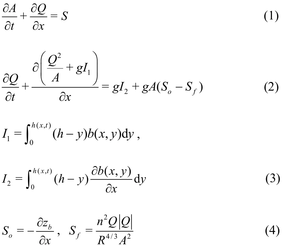
The Saint-Venant equations form a system of hyperbolic conservation laws with eigenvalues and eigenvectors as given by Eqs. (5) and (6) respectively,whereuis the averaged cross-sectional velocity,cis the shallow water wave celerity, andBis the channel width at the water surface. The momentum equation can be simplified following the Leibniz’s rule and can be written as Eq. (7). The water surface elevation is given byZ=(h+zb).

2. Numerical solution
The proposed SIFD-FVM method solves the continuity equation with the mass-conservative cell centered finite volume method and solves the momentum equation with the semi-implicit finite difference method. The 1-D domain is discretized intoNenon overlapping cells (xi-1/2,xi+1/2)of mesh size of Δxi=xi+1/2-xi-1/2withNe+1 edges (xi±1/2are the locations of cell edges). A sketch of the finite volume cells used is shown in Fig.1.
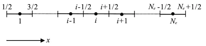
Fig.1 Computational domain and boundary conditions
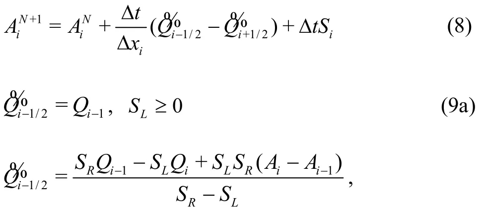
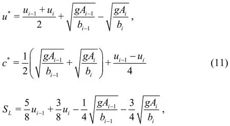
Integrating the continuity equation over theithcell with first-order approximation, and applying the Green’s theorem yields Eq. (8), where Δt=tN+1-tNis the time step size (superscriptsNandN+1 denote current time step and next time step),andare the numerical fluxes at edges of the cell.The Harten-Lax-van Leer (HLL) approximate Riemann solver[31]is used to calculate the numerical flux as shown in Eq. (9). The wave speeds (SL,SR)are given by Fraccarollo and Toro[32]and are shown in Eq. (10), whereu*andc*are given by Eq. (11).To increase the computational efficiency, the wave speeds are estimated by average instead of the minimum or maximum functions as in Eq. (10),resulting in Eq. (12). Numerical results (shown later)prove that using the wave speeds calculated in Eq. (12)for the HLL solver are accurate and performs similar to Eqs. (10) and (11) but with higher computational efficiency.


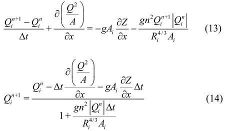
For the discretization of the momentum equation,a procedure similar to the method of lines (MOL) used by Liskovets[33]and Hamdi et al.[34]is adopted. The MOL is regarded as a special finite difference method for solving partial differential equations by discreti zing in all but one dimension and then integrating the semi-discrete system of ordinary equations. Usually,the spatial derivatives are discretized and the time variable are left continuous. Here, the temporal derivative in the momentum equations are discretized first with the semi-implicit scheme as shown in Eq. (13).The variables without superscripts are evaluated at time =Ntt. Note that the diffusion wave model is obtained by ignoring the two terms on the left hand side, while the inertial wave model is obtained by ignoring only the second term on the left hand side of Eq. (13). An explicit solution of the flowrate in the dynamic wave model is obtained by rearranging Eq.(13) as Eq. (14).
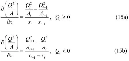
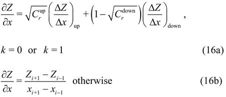
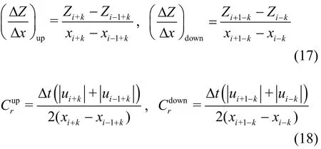
Next, the two spatial derivative terms (convection flux term and surface slope term) in Eq. (14) are evaluated. The momentum flux term is calculated using a simple upwind scheme as shown in Eq. (15),while the surface slope term is calculated using three different schemes. The weighted average water surface gradient approach based on the Courant number and both upwind and downwind slopes[29]for the surface slope term is given by Eq. (16), wherek=0 whenQi>0 andQi-1> 0, andk=1 whenQi< 0 andQi+1<0. The other terms in Eq. (16) are defined in Eqs. (17) and (18). The center difference scheme and the quadratic upstream interpolation for convective kinematics (QUICK) scheme[35]for the water surface slope are given by Eqs. (19) and (20),respectively. As explicit scheme is used in the SIFD-FVM, the time step size should meet the CFL stability requirement given by Eq. (21).


3. Dry bed treatment
For flow between wet cells and dry cells, a sufficiently small dry depthhdry(e.g., 10-8m) is used to check the wetting front and improve numerical stability[19,36]. If the water depth is less thanhdryin a cell, the flow rate is set to zero for that cell. This treatment of dry cell is mass conservative. Numerical tests show that dry depth value affects the time step size. Decreasing the specified dry depth will decrease the time step size required to satisfy the stability requirement[19,29]. For flow over horizontal channels,a very small dry depth value can be used without restricting the time step, while for flow in channels with uneven beds, dry depth of the order of 10-4m is found to avoid the use of extremely small time step size.
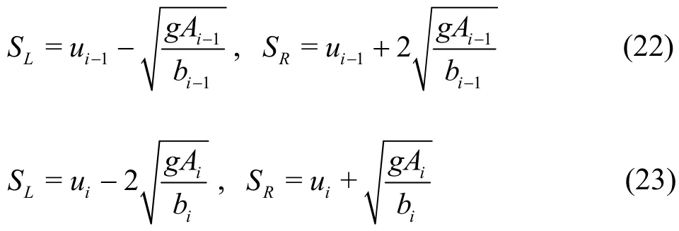
For flow between a wet cell and a dry cell, the wave speeds in the HLL solver at the cell edgei- 1/2 for the dry bed to the right or left are given by Eq. (22) or (23), respectively[31].
4. Boundary conditions
The total number of boundary conditions required for the numerical solution depends on the flow region and regime. At the inflow boundary, one condition (usually discharge) is needed for subcritical flow and two conditions (discharge and flow depth)are required for supercritical flow. For outflow boundary, one condition (usually flow depth) is needed for subcritical flow and none is required for supercritical flow. For subcritical flow, the boundary condition(discharge or flow depth) can be specified at the boundary cells. The ghost cell approach is used for supercritical and open flow boundary conditions[29,36].For supercritical inflow, two ghost cells are introduced in order to specify discharge and flow depth.For supercritical outflow or open outflow boundary,discharge and water level are extrapolated from adjacent interior cells.
5. Evaluation and statistical metrics
The performance of the SIFD-FVM is evaluated in term of accuracy and efficiency. The accuracy of the method is evaluated by comparing the numerical solutions against analytic solutions or available measured data. The efficiency of the method is assessed by comparing with the upwind conservative finite volume method (FVM) developed by Ying et al.[29].The upwind conservative scheme by Ying et al.[29]uses the FVM to solve both continuity and momentum equations with explicit time stepping scheme. The performance of the numerical methods is quantified using the Nash-Sutcliffe efficiency (NSE), percent bias (PBIAS), and ratio of the root mean square error to the standard deviation of measured data (RSR) as suggested by Moriasi et al.[37].
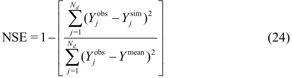
The NSE indicates how well the simulation results versus observed/analytic data fits the line of unit slope and is calculated using Eq. (24), whereis thethjobservation/analytic data,is thejthsimulated value at the same time/location,Ymeanis the mean of the observation/analytic data,andNdis the total number of observation/analytic data. The NSE index ranges between -∞ and 1, with 1 being the optimal value, and values less than 0 indicate unacceptable performance and the mean observed value is a better predictor than simulation.
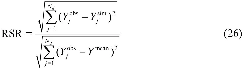
The PBAIS measures the average tendency of model underestimation (PBIAS>0) or model overestimation (PBIAS<0), with optimal value of zero, and is evaluated using Eq. (25). RSR standardizes the root mean square error (RMSE) using the observation standard deviation. RSR ranges between 0 and +∞,with optimum value of 0, and is given by Eq. (26).Note that2
NSE=1-RSR.

The speedup of CPU runtime using SIFD-FVM compared with FVM is evaluated as a ratio of the computer runtimes using FVM and SIFD-FVM.Uniform time steps were used in the following numerical tests for comparison purpose. Note that the time step sizes in following tests gave Courant number much less than unity. As the CPU timer had a resolution of 0.01 s, smaller time steps were used in the numerical tests to give longer CPU times in order to minimize time measurement errors. Both numerical solvers were run on an Ubuntu 12.04 desktop with 3.60 GHz Intel i7 CPU.

Fig.2 (Color online) Numerical and analytic solutions for steady subcritical flow over a bump
6. Numerical tests
The performance of the proposed numerical method is validated through four numerical tests with different flow conditions. Test 1 represents steady flow over a bump for different scenarios, including subcritical flow, supercritical flow, and transcritical flow. Test 2 is an idealized dam-break flow with wet bed or dry bed downstream. Test 3 is a free surface oscillation with moving shoreline in a parabolic bowl.Test 4 and 5 are experimental scale real world problems with irregular channel geometry. Numerical accuracy and speedup of the method are investigated in each of these tests. In the figures and tables, WA,CD, and QK represent discretization of water surface gradient term using weighted average, center difference, and QUICK schemes, respectively.
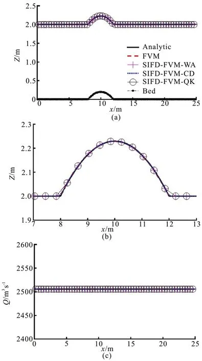
Fig.3 (Color online) Numerical and analytic solutions for steady supercritical flow over a bump
6.1 Test 1: Steady flow over a bump
The numerical scheme was used to simulate steady flows over a bump with three different flow regimes[38]. The frictionless rectangular channel was 100 m wide and 25 m long with uneven channel bed.Mesh size of 0.1 m was used in all three scenarios(subcritical, supercritical, and transcritical). For the subcritical flow, the initial water surface elevation was 0.5 m throughout the channel. Discharge of 18 m3/s at the upstream end and water surface elevation of 0.5 m at the downstream end were specified as boundary conditions. Time step size of 0.01 s was used. The simulated results of water surface elevation and flow rate are shown in Fig.2 for both FVM and SIFD-FVM and compared with the analytic solutions. The water surface elevation is accurately predicted by both FVM and SIFD-FVM. The constant flow rate is better predicted by FVM than SIFD-FVM, as there are sudden changes of flow rate over the bump in the simulated result from SIFD-FVM. The predicted water surface elevations from SIFD-FVM are higher than analytic solution over the bump.
For the supercritical flow case, the initial water surface elevation was 2 m, and the inflow discharge of 2505.67 m3/s and surface elevation of 2 m were specified as boundary conditions at the upstream end of the channel. Time step size of 0.001 s was used.Simulated and analytic results of water surface elevation and flow rate are shown in Fig.3. Water surface level and the constant discharge are well predicted by both FVM and SIFD-FVM.
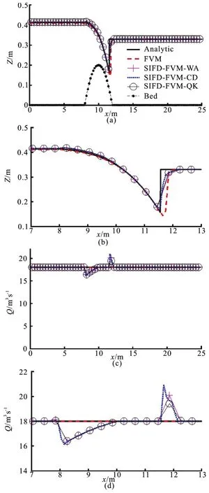
Fig.4 (Color online) Numerical and analytic solutions for steady transcritical flow over a bump

Table 1 Accuracy of numerical simulation in steady flow over a bump

Table 2 Speedup in numerical tests compared with FVM
For the transcritical flow case, the initial water surface elevation was 0.33 m, and inflow discharge of 18 m3/s at the upstream end and water surface elevation of 0.33 m at the downstream end were specified as boundary conditions. The flow regime changed from subcritical flow to supercritical flow and back to subcritical flow with a hydraulic jump over the bump.Time step size of 0.01 s was used. Simulated results of water surface elevation and flow rate for the transcri tical flow case are shown in Fig.4. As in the subcritical case, the constant discharge was better simulated by FVM than SIFD-FVM. However, for the simulated surface elevation, the hydraulic jump was better captured by SIFD-FVM.
The numerical results show that both numerical methods are accurate and robust to simulate different flow regimes. The accuracy of different numerical methods is shown in Table 1 and the speedup using SIFD-FVM is presented in Table 2. The SIFD-FVM achieved speedup of 1.20-1.28 compared to FVM,which means that there is a reduction of run-time by 17%-22%. The center difference scheme is fastest and the weighted average and the QUICK schemes require about the same runtimes. As expected, the FVM results in a better prediction for the flow rate than the hybrid SIFD-FVM. However, the solutions from SIFD-FVM were more accurate in predicting the water depth for the supercritical and transcritical cases.(Slightly higher NSE, lower PBIAS and lower RSR in Table 1).
6.2 Test 2: Idealized dam-break flow with wet or dry beds downstream
An idealized dam-break flood in a rectangular channel was simulated for both wet bed and dry bed downstream. The channel was 1000 m long and 100 m wide with horizontal and frictionless bed. A dam was located at the center of the channel (x=500 m) and removed instantaneously. The initial water level was 10 m upstream for both cases, and 2 m downstream for wet bed case. The total simulation time was 20 s with uniform time step size of 0.001 s, and the mesh resolution was 1 m for both cases. Simulated results of water depth and discharge are shown in Figs. 5, 6 for both wet and dry dam-break cases. Both numerical schemes are able to simulate the dam-break flow over wet and dry bed downstream. The shock wave in wet bed case and the wetting front in dry bed case are simulated accurately. For the depression wave moving upstream, FVM is less diffusive and performed better than SIFD-FVM. For the SIFD-FVM with different schemes for surface gradient, the center difference and QUICK schemes are similar and are less diffusive than the Courant number based weighted average. The center difference and QUICK schemes are also better in predicting the shock wave location in the wet bed case.
The accuracy of the numerical results are presented in Table 3. The speedup achieved using SIFD-FVM are 1.19-1.22 and 1.26-1.28 for the wet and dry cases, respectively (see Table 2). The numerical solutions from FVM were slightly better than SIFD-FVM. From Table 3, the FVM generally gave slightly higher NSE and smaller RSR in water depth prediction compared to SIFD-FVM.
6.3 Test 3: Moving shoreline in a parabolic bowl

Fig.5 (Color online) Numerical and analytic solutions for dam-break flow over wet bed

Fig.6 (Color online) Numerical and analytic solutions for dam-break flow over dry bed
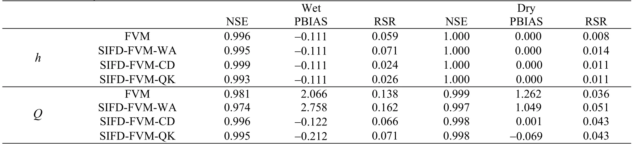
Table 3 Accuracy of numerical simulation in dam-break test
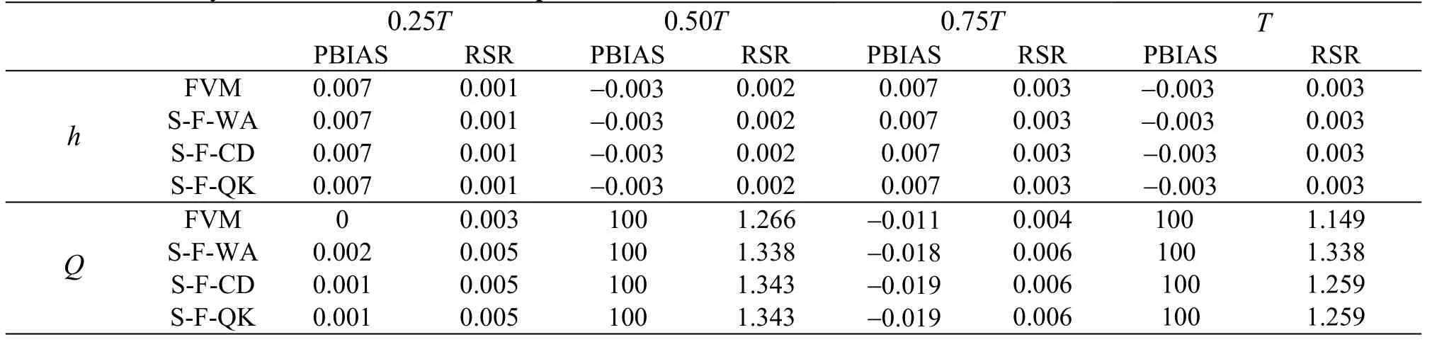
Table 4 Accuracy of numerical simulation in parabolic bowl test
The movement of an oscillating shoreline in a parabolic bowl was simulated and compared to the analytic solutions given by Thacker[39]to test the robustness of the proposed numerical method in modeling wetting and drying over non-uniform slope[19,40]. The analytic solutions of water surface elevation and flow velocity in the rectangular channel with parabolic bed profile are given by Eqs. (27) and(28), respectively, in the region between the moving shoreline, which is given by Eq. (29). The parabolic bed profile and associated parameters are shown in Fig.7

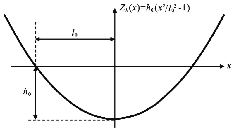
Fig.7 Bed profile in the parabolic bowl test
In the simulation, the following parameters were used:h0=10 m ,l0=600 m , andB=5 m/s, resulting in an oscillation periodT=269s. The parabolic bowl was assumed as a one-dimensional, frictionless channel with uniform width of 100 m, and the computational domain spansx=[-1000,1000] m with uniform mesh size of 1 m. The initial conditions for the water surface level and velocity are given by Eqs. (25) and (26), respectively. With uniform time step of 0.01 s, simulation of one period took 14.74 s for FVM, and took 11.15-11.67 s for SIFD-FVM,resulting in a speedup of 1.26-1.32 (Table 2).

Fig.8 (Color online) Numerical and analytic solutions of surface elevation in test 3
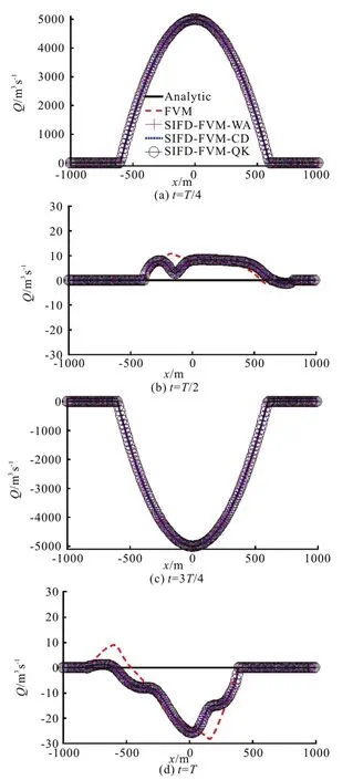
Fig.9 (Color online) Numerical and analytic solutions of flow rate for test 3
The simulated water surface elevation and flow rate at four different times are presented in Figs. 8, 9.The FVM and SIFD-FVM are robust and accurate in modeling wetting and drying process in the parabolic bowl. Both methods give similar accuracy performance as shown in Table 4. Simulation results using FVM performed slightly better than SIFD-FVM in flowrate prediction. The three different schemes for surface gradient discretization in the SIFD-FVM have similar performance as shown in Table 4.
6.4 Test 4: Toce River experimental test
The numerical method was used to simulate the Toce River experimental test presented by Soares-Frazao and Testa[41]. This real world problem was used to test the numerical method with irregular cross sections and non-uniform meshes. The physical model was developed at the ENEL-HYDRO laboratory in Italy and built to 1:100 scale of a reach of the Toce River Valley. Details of the modeling parameters and measurements were provided for numerical simulation of dam-break floods[41,42].
The physical model covered an area of approximately 50 m×12 m with a rectangular tank located at the upstream. The computational domain with 62 cross sections is shown in Fig.10 with five gauge points (P1, P4, P19, P23, and P26). Figure 10 also shows the measured discharge from the upstream tank,which was used in the numerical simulations as a critical inflow boundary condition. The critical flow boundary condition was also applied at the river outlet.The river basin was initially dry. The Manning’s roughness coefficient was taken to be 0.0162 s/m1/3.Uniform time step size of 0.005 s was used in the numerical simulation. The CPU runtime for the FVM was 2.11 s, and 1.74-1.77 s for the SIFD-FVM,resulting in a speedup of 1.19-1.21.
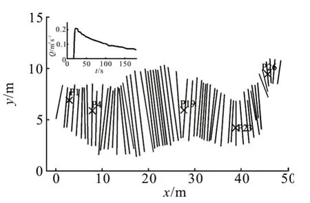
Fig.10 Computational mesh and inflow discharge in Toce River test
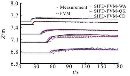
Fig.11 (Color online) Comparison of simulated and measured hydro graphs in Toce River test
The computed and measured stage-time hydro graphs at the five gauges are compared in Fig.11. For the upstream gauges (P1 and P4), the simulated results from both FVM and SIFD-FVM are similar. For the other three downstream gauges, the flood arrival times are better predicted using FVM. Note that with center difference scheme for water surface gradient, there is oscillation at location P26. The simulated and measured maximum water level during the flood are compared in Fig.12. Both methods produce similar prediction of maximum water level except at one downstream section (cross section 56, where the river has a sharp turn), where the predicted maximum elevation from the FVM is higher than measurement,while the predicted maximum elevations from the SIFD-FVM-CD (S-F-CD) and SIFD-FVM-WA (S-FWA) are lower than measurement, the SIFD-FVMQK (S-F-QK) is closest to measurement Accuracy of both numerical methods in predicting the hydro graphs and maximum water level are presented in Table 5.Numerical results from the FVM are generally better than results from SIFD-FVM (smaller PBIAS and RSR) at locations P4, P19 and P23. At gauges P1 and P26, the SIFD-FVM performs better than the FVM.For maximum water elevation prediction, the SIFD-FVM-QK is better than other methods.
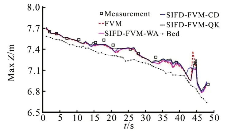
Fig.12 (Color online) Comparison of simulated and measured maximum water levels
6.5 Test 5: Laboratory dam-break flow over a triangular bump
The proposed numerical method is used to simulate a laboratory dam-break flow over a triangular bump proposed by the concerted action on dam break modeling (CADMA) project. This case includes shock wave, wave interaction, and wetting/drying over irregular topography, and is an ideal test to validate the robustness of numerical models[43,44]. The experimental set up of the channel is shown in Fig.13. This rectangular channel is 38 m long, 0.75 m wide with a dam located 15.5 m from the upstream end filling a reservoir with a still water surface elevation of 0.75 m.A symmetric triangular bump (6 m long, 0.4 high)with normal and adverse slopes is installed at 13 m downstream of the dam. In this simulation, the channel downstream of the dam was initially dry. A solid wall no flow boundary condition was applied at the upstream end, while a free outflow boundary condition was applied at the downstream end. A uniform Manning’s roughness coefficient of 0.0125 s/m1/3was used. Simulation was run for 90s after instant dam removal with mesh size of 5 cm and time step size of 0.001 s. The CPU runtime for the FVM was 25.61 s,and 21.02-22.43 s for the SIFD-FVM, resulting in a speedup of 1.14-1.21.
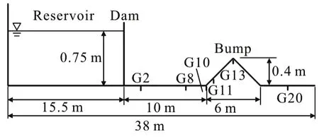
Fig.13 Experimental set up of dam-break flow over a triangular bump
Comparison between simulated and measured hydro graphs at six different gauges (Gauge number denotes distance from the dam, e.g., G2 is 2 m downstream of the dam) are shown in Fig.14 (For clear visualization, results from FVM are not shown).The simulated results using center difference and QUICK schemes for the surface slope agree well with the measured data in flood arriving times and water depths except for small difference at Gauge G20,where flow is complex after the bump and the 1-D assumption may not be suitable. For the simulated results with the weighted average discretization of surface slope (both SIFD-FVM and FVM), the predicted wave arrival times are earlier than measurement. Overall, the new method with center difference and QUICK schemes is able to accurately simulate the flood arrival times, wave interactions,and wet-dry transitions.
6.6 Numerical stability and time-step size
The effect of time-step size on stability for the four numerical tests is also investigated. The maximum time-step allowed and corresponding Courant number (CFL) in these tests are listed in Table 6 for the FVM and SIFD-FVM. For both methods, theeffect of time-step size on stability is case-dependent.Though the explicit scheme requires CFL less than 1,in some cases, the CFL can be larger than 1 as semi-implicit scheme is adopted. For the FVM, the CFL is generally less than 1, except for the supercritical flow over a bump and the idealized dam-break with wet bed downstream, where CFL of 1.41 and 1.38 are used. For the idealized dam-break over wet bed downstream, both methods allow CFL>1. For the SIFD-FVM, CFL can be larger than 1 except in the supercritical flow over a bump (CFL=0.51),dam-break over dry bed (CFL=0.58-0.62), and Toce River test (CFL=0.31-0.43). In the idealized dam-break test and the steady flow over a bump with supercritical flow, the maximum time-step sizes using FVM are larger than using SIFD-FVM. While for other cases, the SIFD-FVM can use larger time-step sizes. In practical applications, numerical methods that allow larger time-steps are preferred. From results in Table 6, the SIFD-FVM is slightly favored over the FVM, as the SIFD-FVM can have CFL>1 in more cases then FVM. For the SIFD-FVM, the three different schemes require about the same maximum time steps, however, the QUICK scheme can use larger time steps in the wet bed dam-break and Toce River tests.
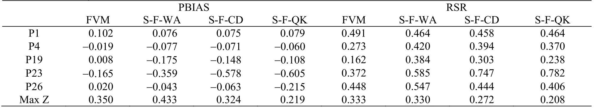
Table 5 Accuracy of numerical simulation in test 4

Fig.14 (Color online) Simulated and measured hydro graphs at different gauges for dam-break flow over triangular bump
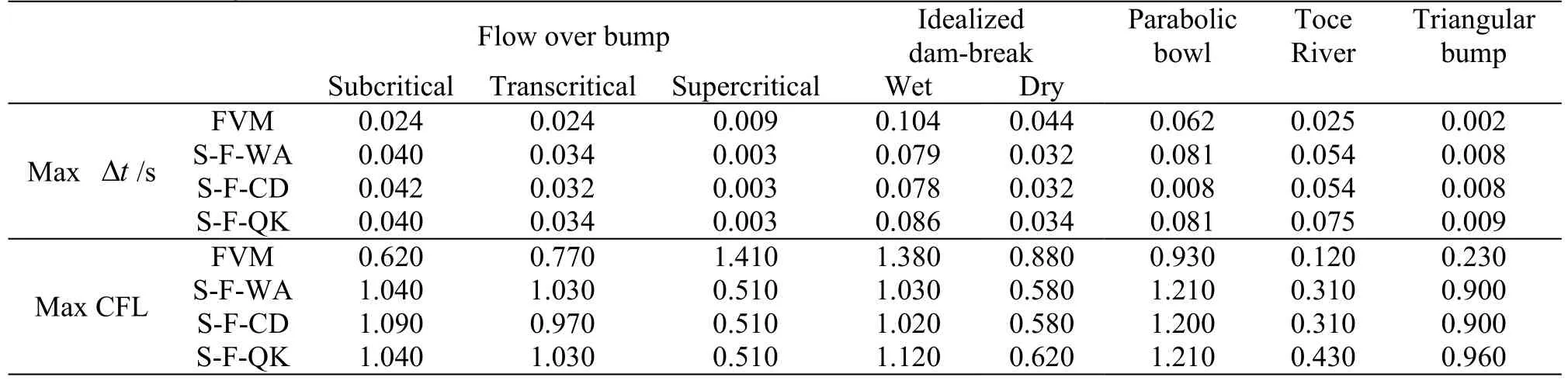
Table 6 Accuracy of numerical simulation in test 4
7. Conclusion and discussion
An efficient and mass-conservative hybrid finite volume/finite-difference method is proposed for the numerical solution of the 1-D Saint-Venant equations in open channel flows. In this method, the continuity equation is discretized using the finite volume method with the HLL approximate Riemann solver, and the momentum equation is solved with a semi-implicit finite difference scheme. An upwind scheme is employed in the spatial discretization of the convective momentum flux term and three schemes are tested for the water surface gradient discretization. The numerical method is demonstrated to be efficient,accurate, and robust in various tests. This method is able to simulate supercritical and transcritical flows,whereas such flows cannot be simulated using simplified models such as the inertial wave model or the diffusive wave model[38]. Both SIFD-FVM and FVM results agree well with the analytic solutions or experimental measurement. NSE was close to the optimal value of one and RSR was close to the optimal value of zero for water depth in the first three idealized tests. As expected, the FVM solutions for the momentum equation were generally more accurate than the SIFD method in predicting the flow rates. For the Toce River test, both methods are considered satisfactory as NSE is greater than 0.75 and RSR is less than 0.60 in the simulated water surface elevation.The SIFD-FVM is 1.19-1.32 times faster than the FVM solver, which means that there is a 16%-24%reduction in runtime without much loss of accuracy in flow rate prediction. The SIFD-FVM is found to be more accurate and efficient with the QUICK scheme for the discretization of the water surface slope. The SIFD-FVM method is attractive and has practical benefit in real world applications where the users are more concerned about computational efficiency and more interested in water surface levels
It is straightforward to extend the SIFD-FVM method for the 1-D Saint-Venant equations to 2-D structured meshes, as the finite difference method can be used for spatial discretization. The hybrid SIFMFVM can also be used in combination with other efficient time-stepping schemes such as the local time-stepping scheme and the adaptive time-stepping scheme to further increase computational efficiency.The FVM solution to the continuity equation can be extended to high-order schemes in space with reconstruction of state variables or using the discontinuous Galerkin method. Additionally, the efficient SIFDFVM method can be applied to other systems including sediment or pollutant transportation, where the FVM is only applied to mass conservation equations,and the momentum equations are solved using the SIFD.
[1] Maleki F. S., Khan A. A., 1-D coupled non-equilibrium sediment transport modeling for unsteady flows in the discontinuous Galerkin framework [J].Journal of Hydrodynamics, 2016, 28(4): 534-543.
[2] Zhang M. L., Xu Y. Y., Qiao Y. et al. Numerical simulation of flow and bed morphology in the case of dam break floods with vegetation effect [J].Journal of Hydrodynamics, 2016, 28(1): 23-32.
[3] Begnudelli L., Sanders B. Unstructured gridfinite-volume algorithm for shallow-water flow and scalar transport with wetting and drying [J].Journal of Hydraulic Engineering,ASCE, 2006, 132(4): 371-384.
[4] Song L., Zhou J., Guo J. et al. A robust well-balanced finite volume model for shallow water flows with wetting and drying over irregular terrain [J].Advances in WaterResources, 2011, 34(7): 915-932.
[5] Ponce V. M. Kinematic wave controversy [J].Journal of Hydraulic Engineering, ASCE, 1991, 117(4): 511-525.
[6] Singh V. P. Kinematic wave modeling in water resources,surface-water hydrology [M]. Chichester, UK: John Wiley and Sons, 1996.
[7] Akan A. O., Yen B. C. Diffusion-wave flood routing in channel networks [J].Journal of Hydraulic Engineering,ASCE, 1981, 107(6): 719-732.
[8] Hromadka T. V., Yen C. C. A diffusion hydrodynamic model (DHM) [J].Advances in Water Resources, 1986,9(3): 118-170.
[9] Defina A., D’alpaos L., Matticchio B. A new set of equations for very shallow water and partially dry areas suitable to 2D numerical models (Molinaro P., Natale L.Modelling of flood propagation over initially dry areas)[M]. New York, USA: American Society of Civil Engineers, 1994, 72-81.
[10] Aronica G., Tucciarelli T., Nasello C. 2D multilevel model for flood wave propagation in flood-affected areas [J].Journal of Water Resources Planning and Management,1998, 124(4): 210-217.
[11] Ponce V. M., Simons D. B., Li R. M. Applicability of kinematic and diffusion models [J]. Journal of Hydraulic Engineering, ASCE, 1978, 104(3): 353-360.
[12] Tsai C. W. Applicability of kinematic, noninertia, and quasi-steady dynamic wave models to unsteady flow routing [J].Journal of Hydraulic Engineering, ASCE,2003, 129(8): 613-627.
[13] Moramarco T., Pandolfo C., Singh V. P. Accuracy of kinematic wave and diffusion wave approximations for flood routing I: Steady analysis [J].Journal of Hydrologic Engineering, 2008, 13(11): 1078-1088.
[14] Lal A. M. W., Toth G. Implicit TVDLF methods for diffusion and kinematic flows [J].Journal of Hydraulic Engineering, ASCE, 2013, 139(9): 974-983.
[15] Ponce V. M. Generalized diffusion wave equation with inertial effects [J].Water Resources Research, 1990, 26(5):1099-1101.
[16] De Almeida G. A. M., Bates P. Applicability of the local inertial approximation of the shallow water equations to flood modeling [J].Water Resources Research, 2013,49(8): 4833-4844.
[17] Neal J., Villanueva I., Wright N. et al. How much physical complexity is needed to model flood inundation [J].Hydrological Processes, 2012, 26(15): 2264-2282.
[18] Liang Q., Chen K. C., Hou J. et al. Hydrodynamic modeling of flow impact on structures under extreme flow conditions [J].Journal of Hydrodynamics, 2016, 28(2):267-274.
[19] Song L., Zhou J., Li Q. et al. An unstructured finite volume model for dam-break floods with wet/dry fronts over complex topography [J].International Journal for Numerical Methods in Fluids, 2011, 67(8): 960-980.
[20] Kesserwani G., Ghostine R., Vazquez J. et al. Riemann solvers with Runge-Kutta discontinuous Galerkin schemes for the 1D shallow water equations [J].Journal of Hydraulic Engineering, ASCE, 2008, 134(2): 243-255.
[21] Lai W., Khan A. A. Modeling dam-break flood over natural rivers using discontinuous Galerkin method [J].Journal of Hydrodynamics, 2012, 24(4): 467-478.
[22] Sanders B. F. Integration of a shallow water model with a local time step [J].Journal of Hydraulic Research, 2008,46(4): 466-475.
[23] Lai W., Khan A. A. A parallel two-dimensional discontinuous Galerkin method for shallow water flows using high-resolution unstructured meshes [J].Journal of Computing in Civil Engineering, 2016, 31(3): 04016073.
[24] Yu H., Huang G., Wu C. Efficient finite-volume model for shallow-water flows using an implicit dual time-stepping method [J].Journal of Hydraulic Engineering, ASCE,2015, 141(6): 04015004
[25] Schippa L., Pava S. Bed evolution numerical model for rapidly varying flow in natural streams [J].Computers and Geosciences, 2009, 35(2): 390-402.
[26] Franzini F., Soares-Frazao S. Efficiency and accuracy of lateralized HLL, HLLS and augmented Roe’s scheme with energy balance for river flows in irregular channels [J].Applied Mathematical Modelling, 2016, 40(17-18):7427-7446.
[27] Burguete J., Garcia-Navarro P. Improving simple explicit methods for unsteady open channel and river flow [J].International Journal for Numerical Methods in Fluids,2004, 45(2): 125-156.
[28] Ying X., Wang S. Improved implementation of the HLL approximate Riemann solver for one-dimensional open channel flows [J].Journal of Hydraulic Research, 2008,46(1): 21-34.
[29] Ying X., Khan A. A., Wang S. S. Y. Upwind conservative scheme for the Saint Venant equations [J].Journal of Hydraulic Engineering, ASCE, 2004, 130(10): 977-987.
[30] Cunge J. A., Holly F. M., Verwey A. Practical aspects of computational river hydraulics [M]. London, UK: Pitman,1980.
[31] Harten A., Lax P. D., Van Leer B. On upstream differencing and Godunov-type schemes for hyperbolic conservation laws [J].SIAM Review, 1983, 25(1): 53-79.
[32] Fraccarollo L., Toro E. F. Experimental and numerical assessment of the shallow water model for two-dimensional dam-break type problems [J].Journal of Hydraulic Research, 1995, 33(6): 843-864.
[33] Liskovets O. A. The method of lines [J].Differential Equations, 1965, 1: 1308-1323.
[34] Hamdi S., Schiesser W. E., Griffiths G. W. Method of lines [J].Scholarpedia, 2007, 2(7): 2859.
[35] Leonard B. P. A stable and accurate convective modeling procedure based on quadratic upstream interpolation [J].Computer Methods in Applied Mechanics and Engineering, 1979, 19(1): 59-98.
[36] Sanders B. F. High-resolution and non-oscillatory solution of the St. Venant equations in non-rectangular and non-prismatic channels [J].Journal of Hydraulic Research,2001, 39(3): 321-330.
[37] Moriasi D. N., Arnold J. G., Van Liew M. W. et al. Model evaluation guidelines for systematic quantification of accuracy in watershed simulation [J].Transactions of the ASABE, 2007, 50(3): 885-900.
[38] Lai W., Khan A. A. Discontinuous Galerkin method for 1D shallow water flow with water surface slope limiter [J].International Journal of Civil and Environmental Engineering, 2011, 75(3): 167-176.
[39] Thacker W. C. Some exact solutions to the nonlinear shallow-water wave equations [J].Journal of Fluid Mechanics, 1981, 107: 499-508.
[40] Xing Y., Zhang X., Shu C. Positivity-preserving high order well-balanced discontinuous Galerkin methods for the shallow water equations [J].Advances in Water Resources, 2010, 33(12): 1476-1493.
[41] Soares-Frazao S., Testa G. The Toce River test case:Numerical results analysis [J].Proceedings of the 3rd CADAM Workshop, Milan, Italy, 1999.
[42] Khan A. A., Lai W. Modeling shallow water flows using the discontinuous Galerkin method [M]. Boca Raton, FL,USA: CRC Press, 2014.
[43] Hiver J. M. Adverse-slope and slope (bump) [C].Concerted Action of Dam Break Modelling: Objectives,Project Report, Test Cases, Meeting Proceedings, Louvain,Belgium, 2000.
[44] Liang Q., Marche F. Numerical resolution of well-balanced shallow water equations with complex source terms[J].Advances in Water Resources, 2009, 32(6): 873-884.
- 水动力学研究与进展 B辑的其它文章
- Numerical analyses of ventilated cavitation over a 2-D NACA0015 hydrofoil using two turbulence modeling methods *
- Couple stress fluid flow in a rotating channel with peristalsis *
- 2-D eddy resolving simulations of flow past a circular array of cylindrical plant stems *
- Revisit submergence of ice blocks in front of ice cover-an experimental study *
- Energy dissipation of slot-type flip buckets *
- Some notes on numerical simulation and error analyses of the attached turbulent cavitating flow by LES *