
Galerkin Finite Element Study on the Effects of Variable Thermal Conductivity and Variable Mass Diffusion Conductance on Heat and Mass Transfer∗
2018-07-09 06:46ImranHaiderQureshiNawazShafiaRanaandZubair
Imran Haider Qureshi,M.Nawaz,Shafia Rana,and T.Zubair
Department of Applied Mathematics and Statistics,Institute of Space and Technology,Islamabad 44000,Pakistan
1 Introduction
Heat and mass transfer is an important mechanism of several industrial and engineering processes.For example,refrigeration,air conditioning,space heating,power generation are well known engineering applications where transfer of heat plays significant role.Beside this,transport of species also occurs in many processes including food processing,oil transport phenomenon and diffusion of certain medicines in blood(drug delivery).Such applications motivate engineers and scientists to investigate the phenomenon of heat and mass transfer both theoretically and experimentally.Theoretical studies in many cases are preferred as these provide sound information without consuming resources in term of money and time.Many theoretical studies on heat and mass are available.However,some recent studies are mentioned here.For instance,Iqbal et al.[1]discussed the transport of heat and mass in magnetohydrodynamic flow of voscoelastic fluid by computing the exact solutions.The effects of dispersion of different nano-sized particles and thermal radiation on heat transfer in hydrodynamic flow of water in the presence of applied magnetic field was studied by Iqbal et al.[2]using shooting algorithm.Theoretical investigation of induced magnetic field on flow of nanofluid is carried out by Iqbal et al.[3]applying Keller Box approach.Mehmood et al.[4]theoretically studied micro-rotation effects(for both weak and strong interactions)on mixed convection flow of Casson fluid over a moving surface.Iqbal et al.[5]numerically analysed the inclined magnetic field on a micropolar Casson fluid flow over a stretching sheet.Iqbal et al.[6]considered nanofluidic transport of gyrotactic microorganisms submerged in water towards Riga plate.Riga plate analysis was carried out by Iqbal et al.[7]employing Keller Box method and shooting technique with Runge-Kutta Fehlberg method of order five.Hayat et al.[8]discussed the effects of temperature and concentration gradients caused by density differences in an axisymmetric flow of second grade fluid by considering constant thermal conductivity and constant mass diffusion coefficient and concluded that the temperature and concentration gradients have significant effects on the transport of mass and heat.Nawaz and Hayat[9]studied transport of nanoparticles in the axisymmetric flow of Newtonian fluid taking diffusion coefficients constant and noted that inclusion of nano-particles enhance the thermal conductivity of the fluid.Nawaz et al.[10]considered thermal diffusion and diffusion thermos effects on transport of heat and mass in axisymmetric flow of second grade fluid taking diffusion coefficients as constant.Tsai and Huang[11]analysed the effect of porous medium on heat and mass transfer in the presence of temperature and concentration gradients taking constant material properties.Beg et al.[12]considered constant diffusion coefficients to investigate thermal diffusion and diffusion thermos effects on the transfer of heat and mass from an isothermal sphere.Simultaneous effects of Newtonian heating on temperature and concentration gradients of Jeffry fluid with constant thermal conductivity are examined by Awais et al.[13]Nadeem and Saleem[14]discussed analytically the effects of nano particles on the conductions of heat transfer in third grade fluid.The effect of Ohmic and viscous dissipation on transfer of heat and mass over a vertical surface were studied by Chen.[15]In studies,mentioned in Refs.[8–15]investigators considered constant diffusion coefficients(thermal conductivity and mass diffusion conductance).However,there are few studies which investigate temperature dependent thermal conductivity.For example,Salahuddin[16]performed numerical study to analyse the effect of variable thermal conductivity on heat transfer in the flow non Newtonian fluid using Keller Box method.Bhuvanavijaya and Malikarjuna[17]studied the effects of variable thermal conductivity on heat and mass transfer in the fluid flow in a rotating system.
Chemical reaction has significant effects on the transport of mass in the fluid flows. The transport rate of mass can be increased/decreased by the constructive/destructive chemical reaction. Several researchers have investigated the effects of chemical reaction on the transport of mass in fluid flows.Some recent studies are mentioned through Refs.[18–20].However it is important to note that,in these studies,[18−20]mass diffusion coefficient is taken constant.
Review of existing literature on the transport of mass and heat in fluid flows reveals that already published work considers diffusion of solute with constant mass diffusion coefficient.No study dealing with both temperature dependent thermal conductivity and concentration dependant diffusion coefficient is available yet.Further,no study considers variable mass diffusion coefficient and variable thermal conductivity simultaneously.Based on this fact,the present investigation has novelty and considers the behaviour of temperature and concentration under variable thermal conductivity and variable diffusion coefficient in the presence viscous dissipation and Joule heating.Dimensionless conservation laws with appropriate boundary conditions are solved numerically by Galerkin finite element method.[21−23]This manuscript comprises of five sections.Mathematical modelling is given in Sec.2.Finite element formulation and assembly process given in Sec.3.In Sec.4 simulated results are discussed.Conclusion is given in Sec.5.
2 Technical Description and Non-Newtonian Rheology
Let us investigate the effects of variable diffusion coefficients(thermal conductivity and mass diffusion coefficient)on the transfer of heat and mass in the flow of Casson fluid over an elastic surface stretching with linear velocity Uw=ar in a radial direction.The elastic stretchable surface is subjected to a constant magnetic field in axial direction.The induced magnetic field is neglected under the assumption of small magnetic Reynolds number.[24]No external electric current is applied.First order chemical reaction is considered.The ambient fluid is also moving in a radial direction with linear velocity Uf=cr.T∞and C∞denote the ambient temperature and concentration respectively.The physical model and coordinate system are given in Fig.1.
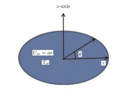
Fig.1 Physical model and coordinates system.
Casson fluid model(non-Newtonian fluid model)characterizes the behaviour of printing inks,food dispersion and chocolate.The constitutive equation of Casson fluid[25−27]is given by
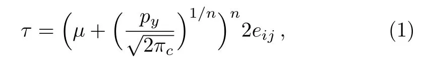
whereµis the plastic dynamic viscosity,eijis the rate of deformation,πcis the critical value of π =eijand pyis the yield stress.For n=1,Eq.(1)becomes
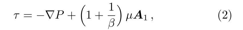
where P is the pressure,is the Casson fluid parameter and A1is the first Revilion-Ericksen tensor defined by A1=gradV+(gradV)t.Analogy between heat and mass transfer are generally governed by general transport convection-diffusion equation.Number of analogies between transport of mass and heat in the flows can be observed. For example first Fick’s Law,J= −D∇C is an analogy of Fourier law of heat conduction q= −k∇T,where D and k,respectively,are diffusion conductance for solute and thermal conductivity of fluid,simultaneously called the diffusion coefficients.These diffusion coefficients,in general,are variable and may be function of temperature,pressure,concentration etc.Through derivation,one can prove that−div(−k∇T)is the amount of heat added to the fluid through conduction and−div(−D∇C)is the amount of solute transported due to concentration differences.This is another analogy between heat and mass transfer.The heat generation and absorption phenomenon is usually formulated by adding the term Q(T−T∞)to the energy equation.First order destructive/constructive chemical reaction is captured by adding the term k(C−C∞)in the mass transport equation.Hence Q(T−T∞)and k(C−C∞)are analogue.These analogies can be proved through derivation of energy and mass transport equations considering heat generation/absorption in heat transfer process and chemical reaction in mass transfer.Studies considering temperature dependent thermal conductivity can be mentioned through Refs.[16–17]and temperature dependent thermal conductivity model used in Refs.[16–17]is given by
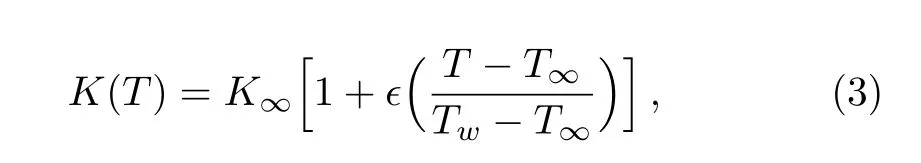
whereis a very small parameter.For=0,Eq.(3)reduces to the case of constant thermal conductivity.In view of several analogies between heat and mass transfer,one can consider the diffusion coefficient D as a linear function of concentration C i.e.
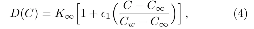
where C∞is the ambient concentration,Cwdenotes the constant concentration at wall and1is a very small parameter.For1=0,Eq.(4)reduces to the case of constant mass diffusion coefficient.
Basic equations of heat and mass transfer in the flow of electrically conducting Casson fluid in the presence of applied constant magnetic field are

where V the velocity of the fluid,d/dt is the material derivative,τ is the stress tensor defined in Eq.(2),ρ is the density of the fluid,σ is the electrical conductivity of the fluid,J is the current density,B is the applied magnetic field,T is the temperature of the fluid,k(T)and D(C)are diffusion coefficients defined in Eqs.(3)and(4),k1is the chemical reaction constant,tr denotes the trace and L=gradV.
For axisymmetric flow,velocity,temperature and concentration fields are

The use of above expressions in Eqs.(5)–(9)gives the following boundary layer equations
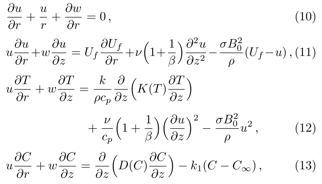
where Ufis the free stream velocity.
No slip at the surface of elastic sheet and state of ambient fluid give the following boundary conditions
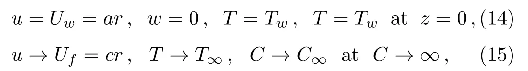
where Uw=ar is the stretching velocity of the elastic surface.
The transformation
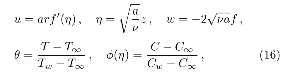
converts Eqs.(10)–(15)to coupled system of nonlinear boundary value problems in the following dimensionless for m
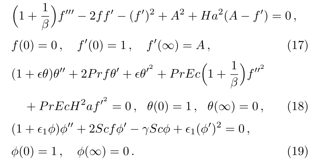
In above equations,Ec=a2r2/cp(Tw− T∞),A=c/a,Sc= ν/D,and γ = k1/c are respectively called Hartmann number,Prandtl number,local Eckert number,stretching parameter,Schmidt number and chemical reaction parameter.It is important to note that boundary value problems(18)and(19)reduce to the classical case of Newtonian fluid of constant thermal conductivity and constant mass diffusion coefficient when=1=0 and β → ∞.
Dimensionless heat flux(Nusselt number)of stretching sheet is defined as
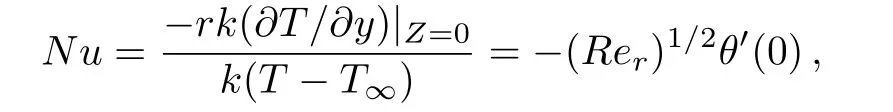
and similarly the dimensionless mass flux(Sherwood number)at the surface of elastic sheet is defined as
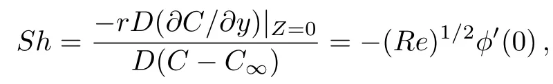
where Rer=(ar2)/ν is the local Reynolds number.
3 Finite Element Formulation
The weighted integral form of residuals for coupled nonlinear system of boundary value problems(17)–(19)over the typical element(ηe,ηe+1)are
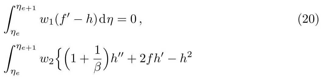
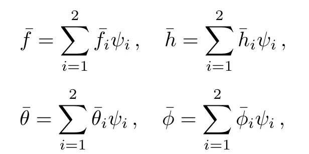
where h=f′and wl(l=1,2,3,4)are the weight functions to minimize the residuals associated with f,h,θ,ϕ.The unknown dependent variables f,h,θ,and ϕ are approximated by the following expansions[22−23]
where fj,hj, θj,and ϕjare the unknown nodal values and ψjare linear shape functions defined by
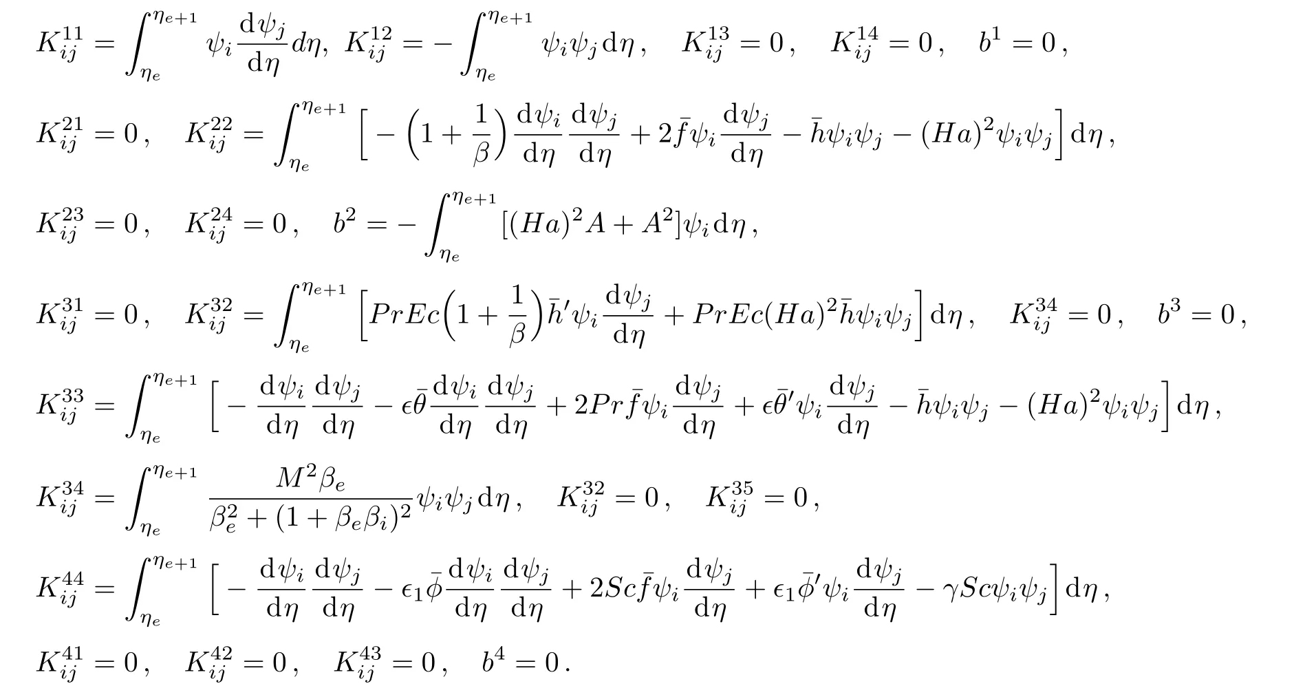
For Galerkin finite element method wl=ψi,i=1,2.[21−23]Substitution of expressions defined by Eq.(24)in residual Eqs.(20)–(23),one can obtain the following stiffness matrices
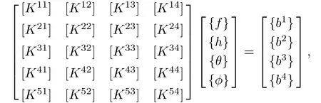
where[Kαξ]and[bα](α = ξ=1,2,3,4)are as follow
After the implementation of assembly process of the elements,we obtain non-linear system of equations.This nonlinear system is linearized by using the following function[22−23]
whereare nodal values at previous iteration.
4 Results and Discussion
The use of finite element formulation of nonlinear boundary value problems gives nonlinear algebraic equations.The coefficients defined above are evaluated for each element and then globalization is performed.The assembled equations are solved iteratively using Picard linearization with computational tolerance 10−8.
4.1 Grid Independent Study
Certain numerical experiments are performed to search infinity physically i.e.to search ηmaxso that asymptotic boundary conditions are satisfied.Performed numerical experiments are recorded in Table 1.This table shows that ηmax=8 where the ambient boundary conditions are satisfied.Hence ηmax=8 is taken as infinity for the coming analysis.The argument of ηmax=8 is also supported by Figs.1–6.The computations become grid independent at 900 elements up to five decimal places(see Table 2).Therefore,forthcoming computations are carried out by discretizing the domain[0,ηmax)into 1000 elements.
Table 1 Numerical values of f′(η),θ(η)and ϕ(η)when Pr=0.72,β =4,= 1=0.8,Ec=1,A=2.5,Sc=1.5,γ=0.5,Ha=1,NE=1000.
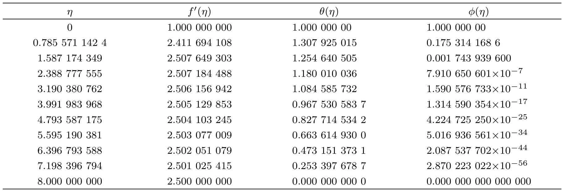
Table 1 Numerical values of f′(η),θ(η)and ϕ(η)when Pr=0.72,β =4,= 1=0.8,Ec=1,A=2.5,Sc=1.5,γ=0.5,Ha=1,NE=1000.
η f′(η) θ(η) ϕ(η)1.000 000 000 1.000 000 00 1.000 000 00 0.785 571 142 4 2.411 694 108 1.307 925 015 0.175 314 168 6 1.587 174 349 2.507 649 303 1.254 640 505 0.001 743 939 600 2.388 777 555 2.507 184 488 1.180 010 036 7.910 650 601×10−7 3.190 380 762 2.506 156 942 1.084 585 732 1.590 576 733×10−11 3.991 983 968 2.505 129 853 0.967 530 583 7 1.314 590 354×10−17 4.793 587 175 2.504 103 245 0.827 714 534 2 4.224 725 250×10−25 5.595 190 381 2.503 077 009 0.663 614 930 0 5.016 936 561×10−34 6.396 793 588 2.502 051 079 0.473 151 373 1 2.087 537 702×10−44 7.198 396 794 2.501 025 415 0.253 397 678 7 2.870 223 022×10−56 8.000 000 000 2.500 000 000 0.000 000 000 0 0.000 000 000 000 000 0
Table 2 Numerical values of f′(η), θ(η)and ϕ(η)for different grid points when Pr=1, β = ∞,= 1=0.8,Ec=1,A=2.5,Sc=1,γ =1,Ha=1.
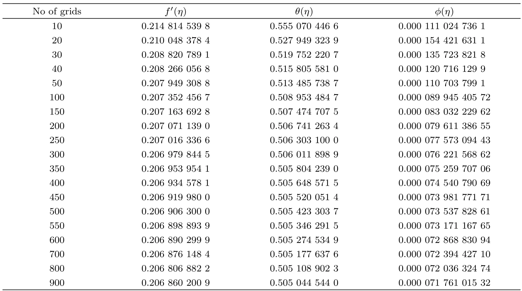
Table 2 Numerical values of f′(η), θ(η)and ϕ(η)for different grid points when Pr=1, β = ∞,= 1=0.8,Ec=1,A=2.5,Sc=1,γ =1,Ha=1.
No of grids f′(η) θ(η) ϕ(η)10 0.214 814 539 8 0.555 070 446 6 0.000 111 024 736 1 20 0.210 048 378 4 0.527 949 323 9 0.000 154 421 631 1 30 0.208 820 789 1 0.519 752 220 7 0.000 135 723 821 8 40 0.208 266 056 8 0.515 805 581 0 0.000 120 716 129 9 50 0.207 949 308 8 0.513 485 738 7 0.000 110 703 799 1 100 0.207 352 456 7 0.508 953 484 7 0.000 089 945 405 72 150 0.207 163 692 8 0.507 474 707 5 0.000 083 032 229 62 200 0.207 071 139 0 0.506 741 263 4 0.000 079 611 386 55 250 0.207 016 336 6 0.506 303 100 0 0.000 077 573 094 43 300 0.206 979 844 5 0.506 011 898 9 0.000 076 221 568 62 350 0.206 953 954 1 0.505 804 239 0 0.000 075 259 707 06 400 0.206 934 578 1 0.505 648 571 5 0.000 074 540 790 69 450 0.206 919 980 0 0.505 520 051 4 0.000 073 981 771 71 500 0.206 906 300 0 0.505 423 303 7 0.000 073 537 828 61 550 0.206 898 893 9 0.505 346 291 5 0.000 073 171 167 65 600 0.206 890 299 9 0.505 274 534 9 0.000 072 868 830 94 700 0.206 876 148 4 0.505 177 637 6 0.000 072 394 427 10 800 0.206 806 882 2 0.505 108 902 3 0.000 072 036 324 74 900 0.206 860 200 9 0.505 044 544 0 0.000 071 761 015 32
4.2 Error Analysis and Convergence
The error defined by
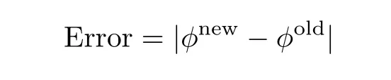
is plotted verses number of iterations in Fig.2.Figure 2 depicts that errors are decreasing functions of number of iterations.The dimensionless radial velocity f′(η),temperature θ(η)and concentration ϕ(η)for different number of elements are plotted in Figs.3–5 respectively.Solution curves become smooth as number of elements is increased(see Figs.3–5).These figures reflect that as number of elements NE is greater than 41,solution curve become smooth.This shows that computed results are going to be grid independent as number of elements are increased.
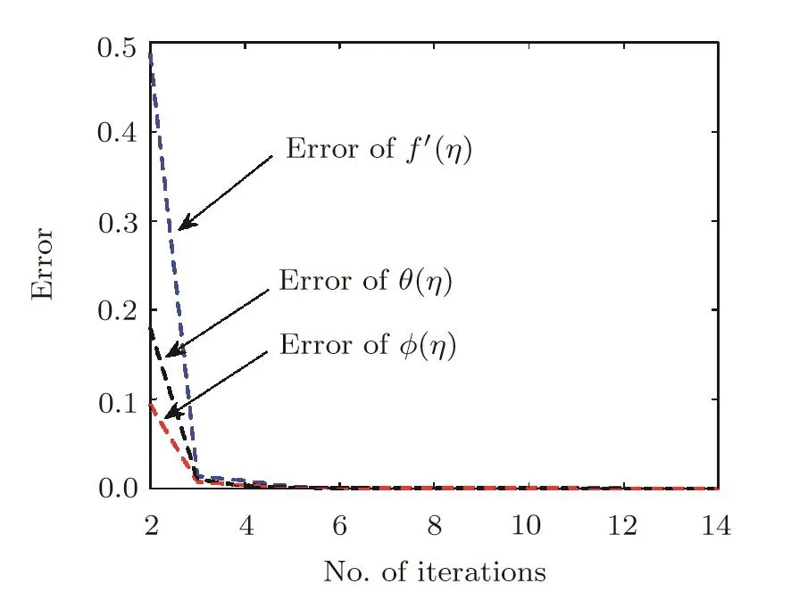
Fig.2 Error verses number of iterations,when A=0.1,Pr=1,β = ∞,= 1=0.8,Ec=0.1,Sc=1,γ=0.5,Ha=1.
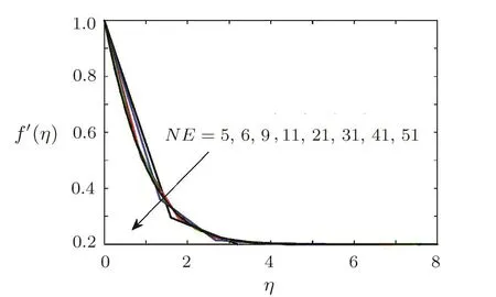
Fig.3 Radial velocity curves for f′(η)at when A=0.2,Pr=0.3,β =1,= 1=0.2,Ec=0.1,Sc=1,γ =0.5,Ha=1.
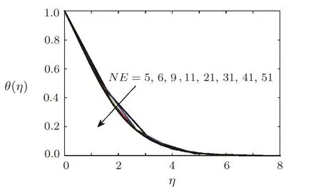
Fig.4 Temperature curves for θ(η)at different grid sizes,when A=0.2,Pr=0.3,β =1,= 1=0.2,Ec=0.1,Sc=1,γ=0.5,Ha=1.
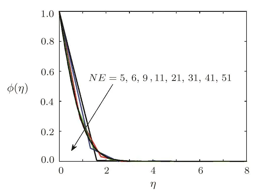
Fig.5 Concentration curves for ϕ(η)at different grid sizes,when A=0.2,Pr=0.3,β =1,= 1=0.2,Ec=0.1,Sc=1,γ=0.5,Ha=1.
5 Results Validation
Computed results are also validated by comparing them with already published results for special case i.e.β→∞(Newtonian fluid case).This comparison is recorded in Table 3. This table shows that an excellent agreement between the already published work and present results.
Parametric studyIn order to explore the physics of the problem,dimensionless radial velocity,temperature and concentration of solute are displayed verses different values of dimensionless parameters β,A,Ha,,Ec,Pr,Sc,γ,and1as shown in Figs.6–12 respectively.
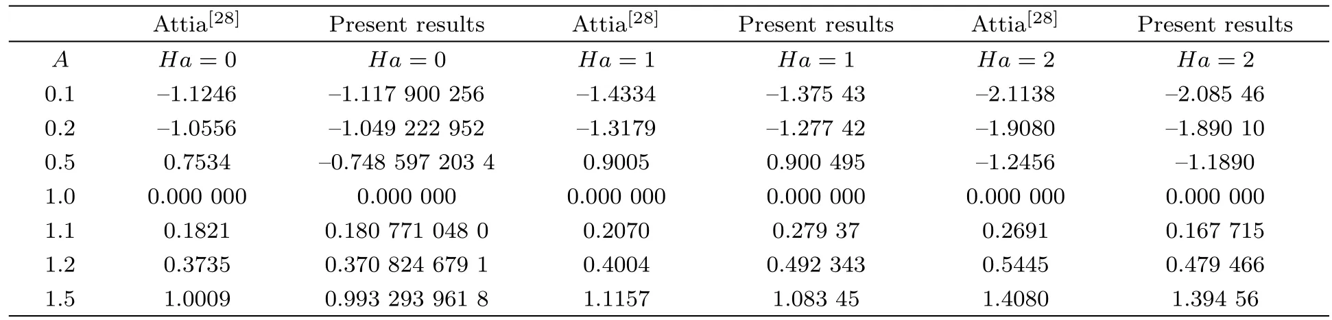
Table 3 Results validation of f′′(0)for different values of A and Ha when β → ∞ (Newtonian fluid).
Effect of Casson fluid parameter β on dimensionless radial velocityFigure 6 is sketched to examine the effect of Casson fluid parameter β on f′(η).Figure 6 reflects that velocity of non-Newtonian fluid is greater than that of Newtonian fluid(β → ∞).Momentum boundary layer thickness is increased by increasing Casson fluid parameter β.
Effect of stretching parameter A on dimensionless radial velocityThe stretching parameter A=a/c,the ratio of stretching velocity Uw=cr to the radial velocity Uw=ar of the ambient fluid A>1,this is the case when stretching velocity is greater than the velocity of ambient fluid and vice versa for A<1.A=1 is the case when both of the velocities are of same order of magnitude.The effect of stretching parameter A is given in Fig.7.Figure 7 shows that for the case when ambient velocity is dominant,radial velocity f′(η)in boundary layer regime decreases by increasing the stretching parameter A.
Effect of Hartmann number on dimensionless radial velocityThe effect of magnetic field on the radial velocity of fluid is noted in Fig.8.Figure 8 illustrates that the radial velocity component decreases by increasing the intensity of magnetic field.This is because of the fact that Lorentz force is opposing force and retards the flow in the radial direction.
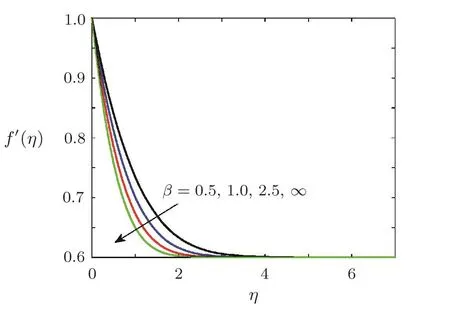
Fig.6 Variation of radial velocity f′(η)against different values of Casson fluid parameter β,when A=0.6,Pr=0.5,β = ∞,=0.2,1=0.5,Ec=0.5,Sc=0.5,γ=0.5,Ha=0.5.
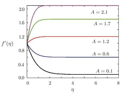
Fig.7 Variation of radial velocity f′(η)against stretching parameter A when Pr=0.7,=0.2,1=0.5,Ec=0.5,β =3,Sc=0.7,γ=0.5,Ha=0.5.
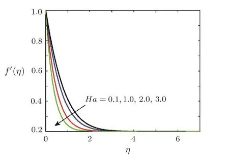
Fig.8 Variation of radial velocity f′(η)against Ha,when Pr=0.7, =0.2,1=0.5,Ec=0.5, β =3,Sc=0.7,γ=0.5,Ha=0.5,A=0.2.
Effect of parametereon temperatureFigure 9 represents the behaviour of dimensionless temperature θ(η)under the variation of parameter.A significant increase in the temperature is noted whenis increased.It is also noted that temperature of the fluid for the case of constant thermal conductivity(=0)is less than that of the fluid with variable thermal conductivity(0).Thermal boundary layer thickness increases significantly when parameteris increased.It is also observed that thermal boundary layer thickness for the case of fluid of constant thermal conductivity is less than that of fluid with variable thermal conductivity.
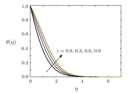
Fig.9 Effect of variation of thermal conductivity on temperature θ(η),when Pr=0.7,Ha=0.5, 1=0.5,Ec=0.1,β=3,Sc=0.7,γ=0.5,Ha=0.5,A=0.2.
Effect of Eckert number on temperatureThe effect of Eckert on temperature θ(η)is displayed in Fig.10.Figure 10 shows that there is a significant increase in temperature when Eckert number Ec is increased.This increase in temperature is obvious because Ec appears as coefficient of viscous dissipation and Joule heating terms(see second last and last term of Eq.(18)).It means that role of Eckert number is two fold i.e.(i)An increase in Ec corresponds to the case when more heat dissipates due to friction force(viscous force)and this dissipated heat adds to the fluid,consequently,temperature of the fluid increases,(ii)Since fluid is electrically conducting and flow is in the presence of magnetic field so current produce as a result of change of magnetic flux.Due to Joule heating phenomenon,some of the electrical energy converts into heat and fluid temperature rises.As Ec is the coefficient of Joule heating term and an increase in Eckert number,to correspond to an increase in Joule heating.Obviously temperature increases.These expectations are well supported by the computed results(see Fig.10).Thermal boundary layer thickness is greatly affected by viscous dissipation and Joule heating phenomena.Figure 10 reveals that boundary layer thickness increases as Ec is increased.Ec=0 is the case when viscous dissipation and Joule heating effects are insignificant.Figure 10 also shows that temperature of fluid for which viscous dissipation and Joule heating are insignificant is less than the temperature of the fluid for which viscous dissipation and Joule heating are significant.From practical point of view,to control thermal boundary layer thickness in magnetohydrodynamic(MHD) flow situations,Casson fluid with negligible viscous dissipation and Joule heating will be more appropriate.
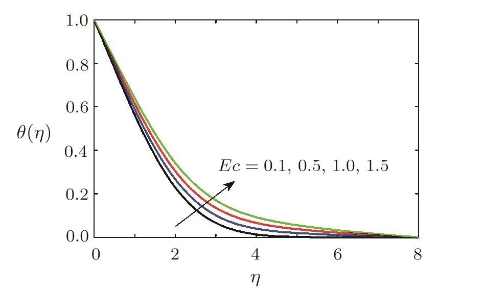
Fig.10 Variation of dimensionless temperature θ(η)against different values of Eckert number Ec when Pr=0.3,Ha=0.5,=0.2,1=0.2,β =3,Sc=0.3,γ=0.5,A=0.6.
Effect of Prandtl number ProntemperatureBehavior of dimensionless temperature under variation of Prandtl number is illustrated by Fig.11.Fluid cools down when Prandtl number is increased because heat diffuse faster due to fast diffusion of momentum.Figure 11 also demonstrates that thermal boundary layer thickness reduces when Prandtl number is increased.
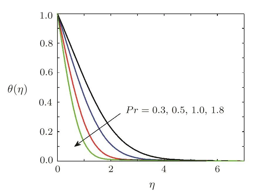
Fig.11 Variation of dimensionless temperature θ(η)against different values of Prandtl number Pr when Ec=0.1,Ha=0.5,=0.2,1=0.2,β =3,Sc=0.7,γ=0.5,A=0.6.
Effect of Schmidt number on concentration of soluteThe variation concentration of the solute in the fluid with variation of Schmidt number is examined and is shown in Fig.12.Figure 12 reveals that concentration increases when the Schmidt number Sc is increased and so is the concentration boundary layer thickness.
Effect of variable diffusion coefficient on concentration of soluteThe effect of variable diffusion coefficient on the concentration of solute is depicted by Fig.13.From Fig.13 it can be seen that concentration of diffusing specie has an increasing behaviour under diffusion coefficient.Consequently,the concentration boundary layer thickness increases when1is increased.
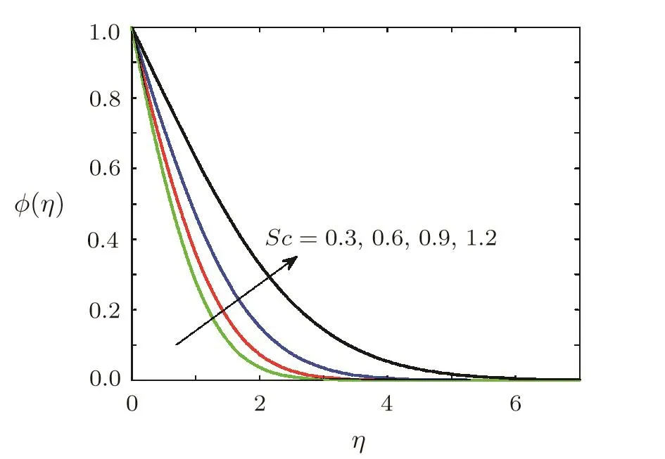
Fig.12 Variation of ϕ(η)against different values of Schmidt number Sc when Ec=0.5,Ha=0.5,=0.2,1=0.5,β =3,Pr=0.5,γ =0.5,A=0.2.
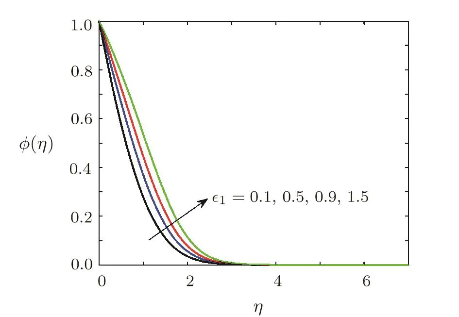
Fig.13 Effect of variation of mass diffusion coefficient on concentration ϕ(η)when Ec=0.1,Ha=0.5,Sc=0.7,=0.2,β =3,Pr=0.7,γ=0.5,A=0.6.
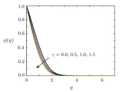
Fig.14 Effect of destructive chemical reaction parameter γ on concentration ϕ(η)when Ec=0.1,Ha=0.5,Sc=0.7,=0.2,1=0.5,β =3,Pr=0.7,A=0.6.
Effect of chemical reaction on concentration of soluteThe effects of first order chemical reaction on the concentration of solute molecules are displayed in Figs.14 and 15.Figure 14 shows the variation of concentration for the case of destructive chemical reaction,whereas influence of constructive chemical reaction is given in Fig.15.Figure 15 shows the concentration of solute molecules decreases when chemical reaction parameter γ (γ >0)is increased as solute molecules are consumed in destructive chemical reaction.The behavior of concentration for the case of constructive chemical reaction(γ<0)is opposite to behavior of concentration in destructive chemical reaction.The influence of stretching ratio parameter A on the concentration of solute is sketched in Fig.16.It is obvious from Fig.16 that concentration decreases when A is increased.It is also clear from Fig.16 that concentration boundary layer thickness is decreased by increasing A.
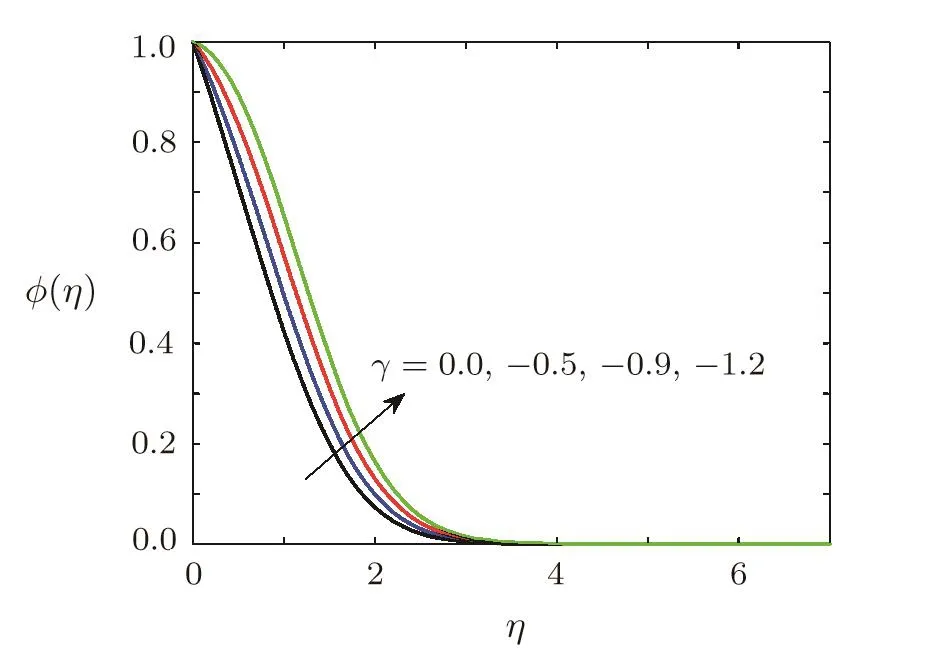
Fig.15 Effect of generative chemical reaction parameter γ on concentration ϕ(η)when Ec=0.1,Ha=0.5,Sc=0.7,=0.2,1=0.5,β =3,Pr=0.7,A=0.6.
Behavior of skin frictionThe behavior of shear stress at the surface of elastic sheet at the surface of the elastic sheet is examined by varying the Casson fluid parameter β and Hartmann number Ha.This behavior of shear stress is recovered in Table 4.It can be observed from this table that shear stress at the surface decreases when Hartmann number Ha and the Casson fluid parameter β is increased.It is also obvious from Table 4 that the shear stress for Casson fluid is less than for the Newtonian fluid.
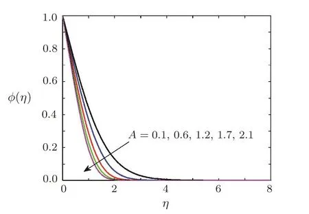
Fig.16 Effect of stretching parameter A on concentration when Pr=0.7,=0.2,1=0.5,Ec=0.5,β =3,Sc=0.7,γ=0.5,Ha=0.5.
Behavior of rate of heat transferThe Nusselt number is the dimensionless form of rate of heat transfer at the sheet and its behavior with respect to the variation of the Casson fluid parameter β and the parameteris represented in Table 5.It is found from Table 5 that the rate of heat transfer decreases when the thermal conductivity of the fluid varies with respect to the temperature.The rate of heat transfer at elastic surface is also decreased when the Casson fluid parameter β is increased.
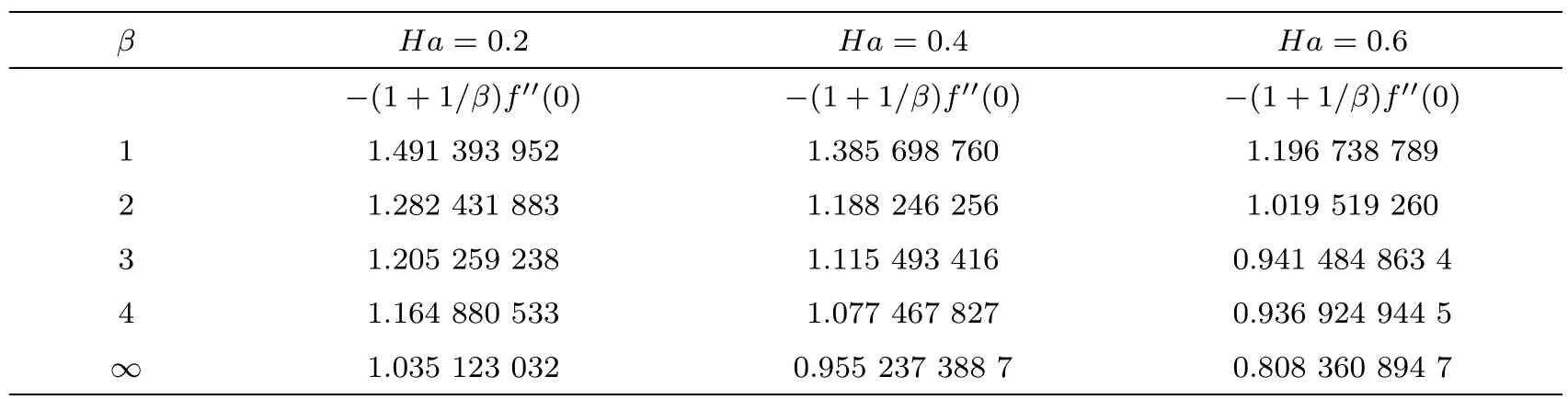
Table 4 Behavior of skin friction coefficient(Rer)−1/2Cf= −(1+1/β)f′′(0)for different values of Casson fluid parameter β and Ha when A=0.1.
Table 5 Behavior of Nusselt number(Rer)−1/2Nu= −θ′(0)for different values of Casson fluid parameter β and when Pr=Ha=Ec=0.1.
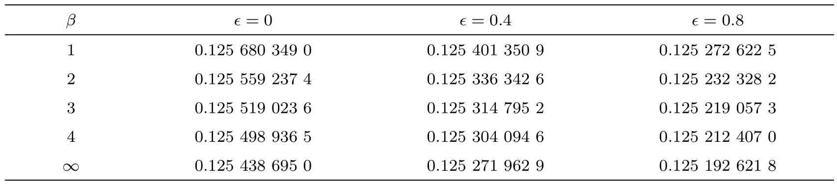
Table 5 Behavior of Nusselt number(Rer)−1/2Nu= −θ′(0)for different values of Casson fluid parameter β and when Pr=Ha=Ec=0.1.
β =0 =0.4 =0.8 0.125 680 349 0 0.125 401 350 9 0.125 272 622 5 2 0.125 559 237 4 0.125 336 342 6 0.125 232 328 2 3 0.125 519 023 6 0.125 314 795 2 0.125 219 057 3 4 0.125 498 936 5 0.125 304 094 6 0.125 212 407 0∞0.125 438 695 0 0.125 271 962 9 0.125 192 621 8 1
Effect of chemical reaction on mass fluxThe effect of variation of diffusion coefficient and first order chemical reaction on mass transport rate(Sherwood number)is given in Table 6.Table 6 represents the variation of Sherwood number as the mass diffusion coefficients increases.It is clear that the Sherwood number decreases when mass diffusion coefficient is increased.Alternatively,mass diffusion rate of solute particles decreases with an increase in the mass diffusion coefficient.Sherwood number increases when chemical reaction parameter γ(γ >0)is increased.However opposite trend is noted for the case of constructive chemical reaction(γ<0).
Table 6 Behavior of Sherwood number(Rer)−1/2Sh= −ϕ′(0)for different values of γ and 1 when Sc=0.1.
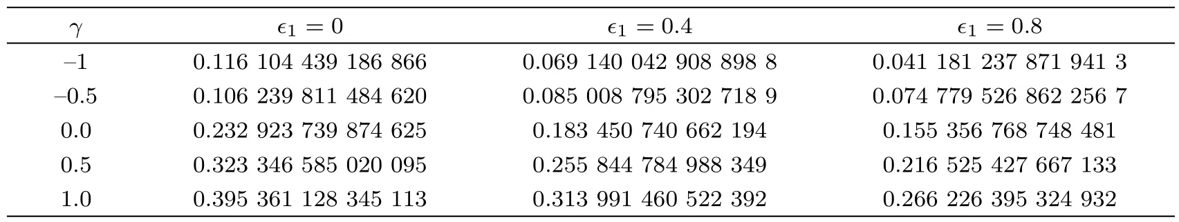
Table 6 Behavior of Sherwood number(Rer)−1/2Sh= −ϕ′(0)for different values of γ and 1 when Sc=0.1.
γ 1=0 1=0.4 1=0.8–1 0.116 104 439 186 866 0.069 140 042 908 898 8 0.041 181 237 871 941 3–0.5 0.106 239 811 484 620 0.085 008 795 302 718 9 0.074 779 526 862 256 7 0.0 0.232 923 739 874 625 0.183 450 740 662 194 0.155 356 768 748 481 0.5 0.323 346 585 020 095 0.255 844 784 988 349 0.216 525 427 667 133 1.0 0.395 361 128 345 113 0.313 991 460 522 392 0.266 226 395 324 932
6 Conclusion
The transport of mass and heat in fluid flows reveals that already published work considers diffusion of solute with constant mass diffusion coefficient.No study dealing with both temperature dependent thermal conductivity and concentration dependant mass diffusion coefficient is studied yet.This study fills this gap.Present work also considers variable mas diffusion coefficient and variable thermal conductivity simultaneously.Based on this fact,the present investigation has novelty and considers the behaviour of temperature and concentration under variable thermal conductivity and variable mass diffusion coefficient in the presence viscous dissipation and Joule heating.Some of the observations from this study are listed below:
(i) Temperature of the Casson fluid(β0)with variable thermal conductivity is high as compare to the Casson fluid with constant thermal conductivity.Thermal boundary layer thickness has an increasing trend as the parameteris increased(increase incharacterises the change in thermal conductivity).Moreover,variation in thermal conductivity causes a significant change in the temperature and the boundary layer thickness.Heat transfer can be enhanced through using fluid with variable thermal conductivity rather than fluid with constant thermal conductivity.
(ii)Mass transport phenomenon can be increased using solute of variable diffusion coefficient rather than solute of constant diffusion coefficient.
(iii) Joule heating and viscous dissipation have vital role in the enhancement of transport of heat.Thus fluid exhibiting viscous dissipation and Joule heating have higher temperature than the fluid having negligible viscous and Joule heating dissipation effects.
(iv)Due to analogy between heat conduction and diffusion of solute(due to concentration differences),the effect of Prandtl number on temperature is similar to the effect of Schmidt number on concentration of solute.
(v)Shear stresses at the surface of stretching sheet have tendency to increase as the Casson fluid parameter β is increased.It is also noted that stretching surface experiences more stresses in case of Casson fluid as compared to the stresses in case of Newtonian fluid(β→∞).Moreover,stresses at the surface of stretching sheet are decreased by increasing the intensity of magnetic field because flow is opposed due to opposing Lorentz force and due to retardation stresses at the surface increases.
(vi)Nusselt number increases with an increase in the Casson fluid parameter β.Similar observations are noted when parameteris increased.Nusselt number of Newtonian fluid is less than that of the Casson fluid(non-Newtonian fluid).
(vii)Sherwood number decreases when mass diffusion coefficient is increased.Alternatively,the rate of diffusion of solute particles in fluid decreases with an increase in the mass diffusion coefficient.Sherwood number increases in case of destructive chemical reaction.However,opposite trend is noted for the case of constructive chemical reaction.
Acknowledgments
Authors are thankful to the reviewers for their useful comments regarding earlier version of this manuscript.
[1]Z.Iqbal,Z.Mehmood,and B.Ahmad,Commun.Theor.Phys.67(2017)561.
[2]Z.Iqbal,E.N.Maraj,E.Azhar,and Z.Mehmood,J.Taiwan Inst.Chem.Eng.81(2017)150.
[3]Z.Iqbal,R.Mehmood,E.Azhar,and Z.Mehmood,Eur.Phys.J.Plus 132(2017)175.
[4]Z.Mehmood,R.Mehmood,and Z.Iqbal,Commun.Theor.Phys.67(2017)443.
[5]Z.Iqbal,Z.Mehmood,E.Azhar,and E.N.Maraj,J.Molecular Liquids 234(2017)296.
[6]Z.Iqbal,E.Azhar,Z.Mehmood,and E.N.Maraj,Results Phys.7(2017)3648.
[7]Z.Iqbal,E.N.Maraj,E.Azhar,and Z.Mehmood,Adv.Powder Technol.28(2017)2332.
[8]T.Hayat,M.Nawaz,S.Asghar,and S.Mesloub,Int.J.Heat Mass Transfer.54(2011)3031.
[9]M.Nawaz and T.Hayat,Adv.Appl.Math.Mech.6(2014)220.
[10]M.Nawaz,A.Alsaedi,T.Hayat,and M.S.Alhothauli,J.Mech.29(2013)27.
[11]R.Tsai and J.S.Huang,Comp.Mat.Sci.47(2009)23.
[12]O.A.B’eg,V.R.Prasad,B.Vasu,et al.,Int.J.Heat Mass Transfer.54(2011)9.
[13]M.Awais,T.Hayat,M.Nawaz,and A.Alsaedi,Braz.J.Chem.Eng.32(2015)555.
[14]S.Nadeem and S.Saleem,Int.J.Heat Mass Transfer.85(2015)1041.
[15]C.H.Chen,Int.J.Eng.Sci.42(2004)699.
[16]T.Salahuddin,M.Y.Malik,Arif Hussain,et al.,Inf.Sci.Lett.5(2016)11.
[17]R.Bhuvanavijaya and B.Mallikarjuna,J.Navel Archi.Marine.Eng.11(2014)83.
[18]S.Ahmed,J.Zueco,and Luis M.López-González,Int.J.Heat Mass Transfer.104(2017)409.
[19]S.M.M.EL-Kabeir,E.R.EL-Zahar,and A.M.Rashad,J.Comp.Theoret.Nanoscience 13(2016)5218.
[20]Muhaimin,R.Kandasamy,I.Hashim,and A.B.Khamis,Theoret.Appl.Mech.36(2009)101.
[21]J.N.Reddy,An Introdaction to Finite Element Method,Mc Graw Hill,New York(1984).
[22]J.N.Reddy,An Introdaction to Nonlinear finite Elemment Analysis,Oxford University Press,Press Inc.,New York(2005).
[23]M.Nawaz and T.Zubair,Results Phys.7(2017)4111.
[24]G.W.Sutton and A.Sherma,Engineering Magnetohydrodynamic,Mc Graw Hill,New York(1965).
[25]N.T.M.Eldabe and M.G.E.Salwa,J.Phys.Soc.64(1995)41.
[26]I.L.Animasaun,E.A.Adebile,and A.I.Fagbade,J.Nig.Math.Sc.35(2015)1.
[27]S.Mukhopadhyay,P.Ranjan,K.Bahattacharyya,and G.C.Layek,Eng.Phys.Math.4(2013)933.
[28]H.A.Attia,Tamkang J.Sci.Eng.10(2007)11.
 Communications in Theoretical Physics2018年7期
- Communications in Theoretical Physics的其它文章
- Electron Correlations,Spin-Orbit Coupling,and Antiferromagnetic Anisotropy in Layered Perovskite Iridates Sr2IrO4∗
- The Three-Pion Decays of the a1(1260)∗
- A New Calculation of Rotational Bands in Alpha-Cluster Nuclei
- Upshot of Chemical Species and Nonlinear Thermal Radiation on Oldroyd-B Nano fluid Flow Past a Bi-directional Stretched Surface with Heat Generation/Absorption in a Porous Media∗
- Detection of Magnetic Field Gradient and Single Spin Using Optically Levitated Nano-Particle in Vacuum∗
- Transverse Transport of Polymeric Nano fluid under Pure Internal Heating:Keller Box Algorithm