Average cost Markov decision processes with countable state spaces

ZHANG Jun-yu, WU Yi-ting, XIA Li, CAO Xi-ren

(1.School of Mathematics,Sun Yat-Sen University,Guangzhou Guangdong 510275,China;2.School of Business,Sun Yat-Sen University,Guangzhou Guangdong 510275,China;3.Department of Electronic and Computer Engineering,Hong Kong University of Science and Technology,Hong Kong,China)

Abstract:For the long-run average of a Markov decision process(MDP)with countable state spaces,the optimal(stationary)policy may not exist.In this paper,we study the optimal policies satisfying optimality inequality in a countable-state MDP under the long-run average criterion. Different from the vanishing discount approach, we use the discrete Dynkin’s formula to derive the main results of this paper.We first provide the Poisson equation of an ergodic Markov chain and two instructive examples about null recurrent Markov chains,and demonstrate the existence of optimal policies for two optimality inequalities with opposite directions.Then,from two comparison lemmas and the performance difference formula,we prove the existence of optimal policies under positive recurrent chains and multi-chains,which is further extended to other situations.Especially,several examples of applications are provided to illustrate the essential of performance sensitivity of the long-run average.Our results make a supplement to the literature work on the optimality inequality of average MDPs with countable states.

Key words: Markov decision process; long-run average; countable state spaces; Dynkin’s formula; Poisson equation;performance sensitivity

1 Introduction

The Markov decision process (MDP) is an important optimization theory for stochastic dynamic systems and has wide applications; see, e.g. [1-10]. In this paper, we study the long-run average MDP with a countable state space.It is well known that in this problem an optimal policy may not exist,and if it exists,it may be history-dependent, not necessarily a stationary (or else called a Markov)policy.

In the literature, conditions have been found that guarantee the existence of the long-run average optimal policy for MDPs with countable states[7-8,10-12].The existence conditions are usually stated in terms of discounted value functions with the discount factor approaching one. It is also proved that there are average optimal policies for MDPs with countable states for which an optimality inequality, instead of an equality,holds.The approach is presented in details in[10],and it is called the“vanishing discount approach”in[7],and the“differential discounted reward”approach in[8].

In this paper,we use the discrete Dynkin’s formula(e.g.page 122 in[13])to derive the average optimal policy. We observed that the long-run average of a countable MDP does not depend on its value at any finite state, or at any“non-frequently visited”states, which is an important fact studied in the literature[3-4,6,8,14].We construct several examples about null recurrent Markov chains, which motivate the derivation of the strict optimality inequality and optimality equality.We present two comparison lemmas and the performance difference formula via the discrete Dynkin’s formula,which is an important tool to prove the existence of average optimal policies.

The Poisson equation provides a method to solve the long-run average cost,where the existence and properties of its solutions are studied in many literature,for example,refer to page 269 to 303 in[5]which considers the Poisson equation with time-homogeneous Markov chains on a countable state space.Actually,the Poisson equation is a different view to study the existence of the long-run average optimal policy. From the Poisson equation, we derive the optimality inequality/equality and the existence of average optimal policies of positive recurrent chains,multi-chains and other generalized forms such as considering the performance sensitivity.One of the optimality inequality directions is presented as the sufficient condition for average optimal. The more general optimality equations are obtained by the approach of performance difference formulas,which is a useful approach beyond the dynamic programming and has been successfully applied to many problems(e.g.[15-16]).

The remainder of this paper is organized as follows.In Section 2,we introduce the optimization problem and derive the Poisson equation of ergodic Markov chains.In Section 3,we give two examples to demonstrate the existence of the long-run average optimal policy for two optimality inequalities with opposite directions.Our main results are given in Section 4,where the existence of optimal policies under multi-chains, null and positive recurrent chains are provided and some examples and applications are also presented. Finally, we conclude this paper in Section 5.

2 Preliminaries

2.1 The problem

At stateiwith actionαdetermined by policyd, a cost (or reward), denoted byCα(i) orCd(i). The discounted cost criterion with discount factor 0<β< 1 under policydis

2.2 The Poisson equation

Consider a Markov chain{Xk,k= 0,1,···}under a Markov policyd(We omit the superscript“d”,for a generic discussion).Letτ(i,j)=min{t>0:Xt=

withg(0)=g(0,0)=0.g(i),i=0,1,···,is called apotential functionof the Markov chain3In the literature, the solution to a Poisson equation is called a potential function; the conservative law for potential energy holds,see[17]and[4]..And we further assume|g(i)|<∞, i ∈S.

LetA:=P −Ibe the discrete version of the infinitesimal generator, withIbeing the identity matrix.g:=(g(0)g(1)···)T,C:=(C(0)C(1)···)T,ande:=(1 1···)T.

Lemma 1 The potential functiong(i) of a Markov chain,i ∈S, in (2) satisfies the Poisson equationAg+C=ηe.

Proof From(2),we have

On every sample path withX1̸=0(whenX1=0,Lemma 1 is easy to verify sinceτ(i,0) = 1,i ∈S),the Markov chain reaches state 0 from stateX1at time 1 after timeτ(i,0)−1,i.e.,τ(X1,0)=τ(i,0)−1,and the second equality in the above equation holds. Thus,this equation is the Poisson equation

Obviously, the potential function is only up to an additive constant;i.e.,ifg(i),i ∈S,is a solution to the Poisson equation,so isg(i)+cfor any constantc.Any statei ∈Scan be chosen as a reference state and we may setg(i)=0.

Remark 1 For null recurrent Markov chains,τ(i,j) may be infinity, andg(i) in (2) is not well defined. However, in some special cases, there might be some functiong(i)and a constantηsuch that the Poisson equation(3)holds,see Example 1.

3 Examples

To motivate our further research,let us first consider some examples.

Example 1 This is a well-known example[6-8,10]that shows there is an optimal policy for which the optimality equation for finite chains does not hold, instead, it satisfies an inequality. As in the literature, we use the discounted performance to approach the longrun average.

4The theory for multi-class decomposition and optimization for finite Markov chains is well developed,see[4,8]for homogeneous chains,and[3]for nonhomogeneous chains.The decomposition of countable state chains is similar to that for the finite chains,except that there are infinitely many sub-chains.

This is called the optimality inequality for the longrun average MDP with countable states in the literature.

Example 2 In this example, we show that the direction of the “optimality inequality” (6) can be reversed.Consider the same Markov chain as Example 1,but with a different cost at statei= 0. Specifically,there are two actions,aandb, having the same transition probabilities at all statesi ∈S,and the same costsC(i) = 1, for alli ̸= 0. However, we setCa(0) = 2 andCb(0) = 3. Policyftakes actionaand policydtakes actionbati=0.

First, we haveηfβ(i)<ηdβ(i). Thus,dis not discount optimal for allβ ∈(0,1). Next, because both Markov chains underfanddare null recurrent,the cost change at one state 0 does not change the long-run average. In general, the long-run average of a stochastic chain does not depend on its values in any finite period or any “zero frequently” visited period [3]. This is called the “under-selectivity” [3,14]. Thus, we haveηf(i)=ηd(i)≡η=1 for alli.Thereforefanddare both long-run average optimal.

Compared with the optimality inequality(6),the inequality sign is reversed in(8).

Remark 2 1) The two inequalities (6) and (8)are not necessary conditions. Also, an average optimal policy may not be the limiting point of discount optimal policies. In the following, we will see that(8)is a sufficient condition for average optimal,and(6)is neither necessary,nor sufficient.

2) In the examples, the Markov chain is null recurrent. So the probability of visiting each state is zero. Therefore, we may arbitrarily change the cost at any state without changing the long-run average; but it changes the relation in the optimality condition.The inequality (6) is due to the null recurrency of the states and the under-selectivity of the long-run average, it is not an essential property in optimization.

4 Optimization in countable state spaces

4.1 Fundamental results

We assume that the transition probability matrixP= [Pi,j]i,j∈Sdoes not depend on time; i.e., the chainXunder a Markov policy is a time-homogeneous Markov chain.

Letr:S →Rbe a function onS,with E[r(Xn)|X0=i]<∞,i ∈S,n≥1; and we also denote it as a column vectorr:= (r(0)r(1)··· r(i)···)T.For time-homogeneous Markov chains, it holds that E[r(Xn+1)|Xn=i]=E[r(X1)|X0=i].

4) The condition (13) is only sufficient, it is not necessary as shown in Example 1. It may not need to hold at some null recurrent states.

Example 3 It is interesting to note that in Example 2, condition (8) satisfies the optimality inequality(13) for both policiesdandf, and hence it is a sufficient condition forJto be the optimal average. However,in Example 1,the inequality(6)is not a sufficient condition.

For history-dependent policies, it is more convenient to state the comparison lemma for all policies.

Proof For a optimization problem with history dependent randomized policy, we can transform into considering randomized Markov policy,see[8].So the proof can be derived by Lemma 2.

The performance difference formula may contain more information than the above two comparison lemmas. For history-dependent chains, the potentials and Poisson equations are not well studied, and the“lim sup” average does not make sense at transient states,so we have to assume that the limit in(1)exists.

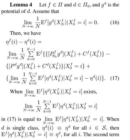
in which the assumption(16)plays an important role in the first equality,then the Lemma follows directly from the Poisson equation ofgd.

4.2 Optimal policy is positive recurrent or multichain

Many results follow naturally from Lemma 2.First,we have

Remark 4 1) In this theorem,d∗cannot be a multi-chain,becauseJin Lemma 3 has to be a constant.For multi-chain optimal policies,see Theorem 3.

2)d∗is usually positive recurrent, but if it is null recurrent and equation(18)holds forηd∗and a functiongd∗,then the theorem may also hold.

3) All the other policiesd ∈Πmay be null recurrent,or multi-chain.Condition(19)may not need to hold at some null states which are null-recurrent at all the Markov chains under all other policies.

Theorem 2 Suppose all policies inΠ0are positive recurrent, and Markov policyd ∈Π0is long-run average optimal inΠ0.Then(18)and(19)hold,and it is optimal inΠ.

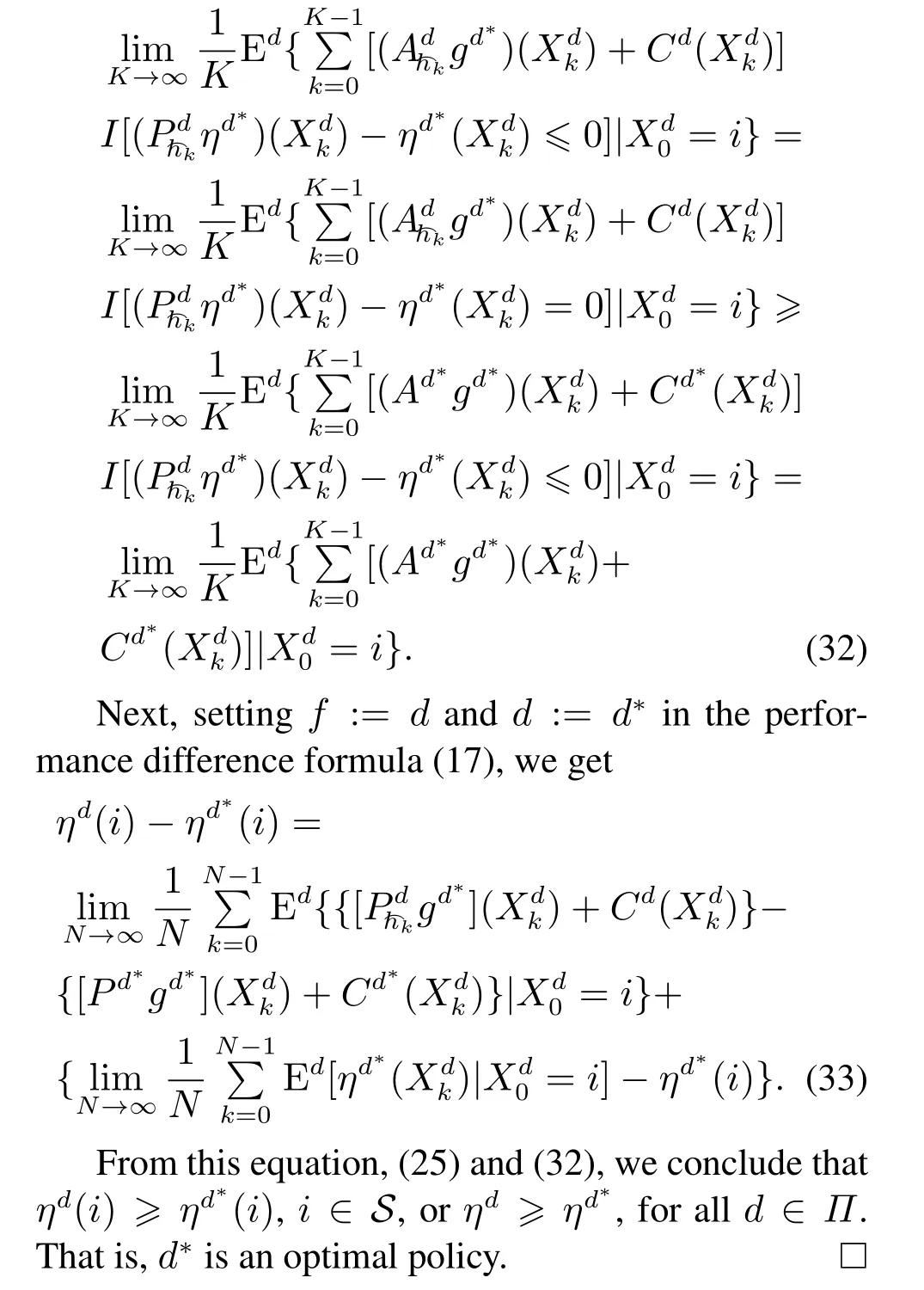
By the performance difference formula (17), we have a set of more general optimality equations. The proof of the following theorem is similar to that in [3]for time nonhomogeneous Markov chains, see also [4]and[8]for finite multi-chains.

Remark 5 1) The restriction of (24) toA0is very important; otherwise, the inequality in (32) may be false and conditions (22) and (24) may not have a solution,see also Example 9.1.1 in[11].

2) The technical conditions (21) and (23) indicate that some kind of uniformity is required for countablestate problems.They are not very restrictive and can be replaced by other similar conditions.

4.3 Under-selectivity

Under-selectivity refers to the property that the long-run average of a stochastic chain does not depend on its value in any finite period, or at any “nonfrequently visited”periods,or states,defined below.

It is clear that non-frequently visited sets include transient states in multi-chains and finite sets of null recurrent states.

Theorem 4 Theorem 3 holds even if Condition(24) does not hold at any non-frequently visited set of states of a policy.

4.4 Null recurrent Markov policies

When the optimal policy is null recurrent,the situation is a bit complicated.The Poisson equation(3)and the potential functiong(i)may not exist,and it is difficult to find the functionr(i),i ∈S,in(13),except for very simple cases,e.g.in Examples 1 and 2,r(i)≡0,for alli ∈S.

This is the “optimality inequality” among these two policies.As explained in Examples 1 and 2,this inequality is due to the null recurrency ofiand the underselectivity of average optimality.In fact,both directions≤and ≥are possible in(35).Whendis also null recurrent,the situation is more complicated because there is no Poisson equation.

Example 4 The structure of the Markov chain is the same as Example 1. The state space isS={0,1,2,···}. At statei≥1, there is a null action withPi,i−1= 1. At state 0, the transition probabilities are given byP0,i> 0,i≥1. We consider two policiesfandd:

5 Conclusion

We summarize this paper with the following observations.

1) The optimality inequality(13)is a sufficient condition for average optimal. The strict inequality may hold at null recurrent states. When the optimal policy is positive recurrent, the inequality becomes an equality.

2) A null recurrent Markov chain visits any state with a probability of zero, so the cost function at such a state can be changed without changing the value of long-run average. Thus, any optimality equality or inequality involving the cost may not need to hold at such a state. In other words, the inequality may be in either direction at a null recurrent state for the optimal policy(see Examples 1 and 2).This is purely the consequence of null recurrency and under-selectivity.

3) The existence of average optimal policies of countable MDPs is mainly derived by the Dynkin’s formula from a view of performance difference.Example 4 shows the application of the main results,which makes a supplement to the existing literature work.