BITS: an efficient transport solver based on a collocation method with B-spline basis

Xiaotao XIAO (肖小涛),Shaojie WANG (王少杰),Lei YE (叶磊),Zongliang DAI (戴宗良),Chengkang PAN (潘成康) and Qilong REN (任启龙)

1 Institute of Plasma Physics,Chinese Academy of Science,Hefei 230031,People's Republic of China

2 Department of Modern Physics,University of Science and Technology of China,Hefei 230026,People's Republic of China

Abstract A B-spline Interpolation Transport Solver (BITS) based on a collocation method is developed.It solves transport equations as a generalized interpolation problem,taking the first-order accuracy in time and the second-order accuracy in space along with a predictor-corrector or under-relaxation iteration method.Numerical tests show that BITS can solve one-dimensional transport equations for tokamak plasma more accurately without additional computation cost,compared to the finite difference method transport solver which is widely used in existing tokamak transport codes.

Keywords: plasma simulation,transport equation,collocation,B-spline,tokamak

1.Introduction

The complexity of transport process in tokamak plasma is generally acknowledged due to various kinds of sources and sinks,instabilities,plasma-surface interactions and so on [1-3].Numerical simulation is an essential tool to understand the transport physics of tokamak plasma.Since the magnetic field in a tokamak has a nested structure,the magnetohydrodynamic equation of particle balance,electron and ion energy conservation,Faraday’s law,toroidal momentum can be simplified to a set of one-dimensional (1-D) flux surface averaged transport equations [4,5].A lot of transport codes have been developed by solving these transport equations since around the 1980s,such as ONETWO [6],TRANSP [7,8],ASTRA [9],and ETS[10].These codes are widely used to interpret experiments at modern tokamaks,such as EAST[11]and HL-2A[12],and help to predict transport of future tokamak devices,such as CFETR[13].In order to simulate all phases of a tokamak scenario,the transport codes are integrated with other tokamak-physics codes.A lot of integrated suites of codes have been developed,such as CRONOS [14],JINTRAC [15],OMFIT [16],IMAS [17]and TRIASSIC [18].

Due to the huge computational resources required by these simulations,it is meaningful to develop an efficient transport solver.Although transport solvers of these codes are firstly and usually developed based on the finite difference method(FDM),different numerical methods continue to be developed to make the transport solver more efficient.For example,the finite element method using a Hermite basis function is applied to solve the current diffusion equation in tokamaks [19].The finite volume method is used in a two-dimensional (2-D) transport solver as it guarantees conservation of the fluxes in both parallel and perpendicular directions [20].Since widely used theorybased transport models such as GLF23[21],MMM95[22]and TGLF [23]have a strong nonlinear dependency on the temperature and density gradients,it is very important to obtain the gradients of physics variables accurately and smoothly.A highorder interpolated differential operation scheme[24]is employed to solve not only the physics variable but also its gradient.It provides an accurate transport solution using a small number of grid points with robust nonlinear convergence.However,this scheme is still under the framework of FDM; the result is improved at the cost of much more computation cost (the gradient of the variable is taken as additional independent variable and a higher-order accuracy formula is used).In this work,a B-spline Interpolation Transport Solver (BITS) is developed to solve the transport equations of tokamak plasma.The computation costs of solving differential equations by FDM and a collocation method are at the same level,while smoother results can be obtained by the collocation method.This helps to reduce the error of numerical results greatly.

In section 2 the transport equations,numerical scheme of the collocation method and FDM,and iteration method are introduced.The results of a few different cases using FDM and the B-spline collocation method are compared in section 3.A conclusion is given in the final section.

2.Description of scheme

The 1-D energy diffusion equation for magnetically confined toroidal plasma in an axisymmetric tokamak can be simplified in cylindrical coordinates as

Here,nis the particle density,Tis the temperature of the electron or ion species,ρ is the normalized minor radius proportional to the square root of the toroidal flux,χ is the effective thermal diffusivity,andSis the source term that includes ohmic heating,ionization,radiation loss,electronion heat exchange,and external auxiliary heating such as neutral beam injection and radiofrequency heating.For a given sourceS(ρ,t),boundary conditionT′ ∣ρ=0=0,T∣ρ=1=Tb,and initial conditionT(ρ,t=0)=T0(ρ),this equation is well posed.The radial coordinate ρ is uniformly divided into grid points ρ1=0,…,ρi,…,ρN=1 for simplicity,i.e.Δρ = ρi+1-ρi= (ρN-ρ1)/(N-1),i= 1,…,N-1.A non-uniform interval is also applicable.Tat time stepnis marked asTn.

2.1.Collocation method

Based on collocation,Tis approximated by a linear combination of basis functionBi,k(ρ).Here the second-order accuracy is used,i.e.T(ρ)=ΣiαiBi,3(ρ).The stable evaluation ofB(ρ)and its derivatives are given in the appendix.It can be simply understood as a generalized piecewise polynomial function.It is nonzero only inksuccessive intervals,and it is actually a polynomial function on each interval.Once grid points are given,and a proper knot sequencet1,…,tN+kis generated,thenBi,k(ρ)is totally determined.In this work,the knot sequence is generated as follows:

in whichMBρis a tridiagonal matrix,with only two additional nonzero elementsm1,3,mN,N-2.Here elementMBρ(i,j) is written asmi,j=Bj(ρi).HereMBρ,MBρ′,MBρ″are all tridiagonal matrices,and only two additional elements are nonzero:the third one in the first row and the third from last one in the last row.Since grid points ρ1,…,ρNand knot sequencet1,…,tN+3remain unchanged after initialization,all the elements of matrixMBρ,MBρ′,MBρ″can be calculated once and used repeatedly.

For interior pointsi=2,…,N-1,the equation is discretized as

It is very easy to implement a higher-order accuracy formula for the collocation method.As shown before,when the second-order accuracy formula is used,kis set as 3,the length of the knot sequence isN+3,andMBρ,MBρ′,MBρ″have three nonzero elements in each row.If we want to use the fourth-order accuracy formula,we simply setkas 5,generate a proper knot sequence with a length ofN+5,and matricesMBρ,MBρ′,MBρ″have five nonzero elements in each row,while all other things remain the same.

2.2.FDM

Employing the backward Euler scheme for time integration,which is the first-order accurate in time,

Based on FDM,the diffusion term is discretized by the second-order center difference as

Inner boundary conditioni=1 is implemented by the second-order forward finite difference formula

Outer boundary conditioni=N,

Finally,equations (16)-(18) constitute a matrix equation,

2.3.Iteration method

The matrix equation (14) derived by the collocation method and equation (19) by FDM can both be written like this:

The predictor-corrector method generally suffers from a large numerical oscillation when coupled to theory-based transport models,such as the stiff transport model.The under-relaxation method and regula-falsi method can overcome this difficulty [24].In this work,the under-relaxation method is applied if the predictor-corrector iteration can hardly converge.The diffusion term is calculated using χn+1,llike this:

in which ϵ is the under-relaxation factor and superscriptlstands for thel-th iteration at each time step.

3.Results

Based on the FDM and collocation method mentioned in the previous section,two solvers(FDMS and BITS)are developed.Their results for different cases are compared in this section.Unless explicitly specified,BITS takes the same second-order accuracy (k=3) in space as FDMS.For the first-order accuracy discretization in time and the second-order accuracy discretization in space,the discretization errors are linear over the time step and quadratic over the space step.Since iteration is usually needed to solve the nonlinear equation (20) for each time step,this brings additional errors.For simplicity,uniform Δρ in the minor radius is used from now on for both solvers;however,a non-uniform interval is also applicable.

3.1.Steady-state transport equation

For the sake of simplicity,densitynand conduction coefficient χ are set as constant.In the steady state,the energy transport equation (1) is simplified as:

whereTi,analyticdenotes the analytic solution ofTat thei-th grid point.

As the grid points in ρ ∈[0,1]increase from 9 to 17,33,65,129,the results of these two solvers both converge.The calculated errors by these two solvers are plotted in figure 1.As a cross-check,the results by Park(figure 2 of[24])are also plotted,in which the cited second-order FDM result is marked as Park_FDM,and the cited fourth-order Interpolated Differential Operator (IDO) scheme result is marked as Park_IDO.Although the IDO method has a fourth-order accuracy,the highest power of the Hermite interpolation function used in equation (2) of [24]is 5,so we compare it to the BITS result withk=6(the highest power of polynomial is 5).Firstly,the results of FDMS developed in this work are as good as the results of the same method developed by Park.Secondly,the results of the fifth-order BITS (k=6,marked as BITSk6) are as good as the results of the IDO method.Finally,the error of the second-order BITS(k=3,marked as BITSk3)is about 1/4 to 1/5 of the error of the second-order FDMS.

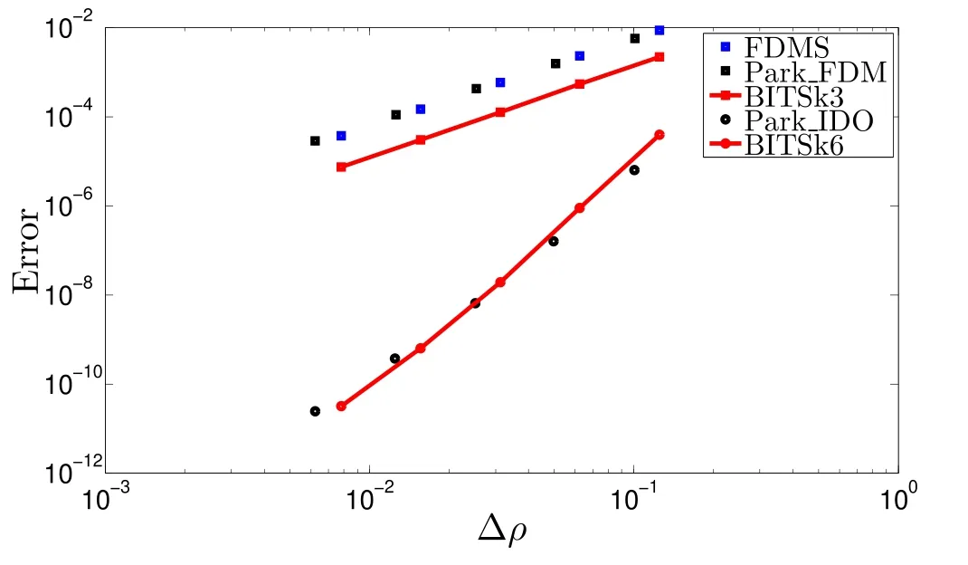
Figure 1.Error of T by different solvers.For the second-order scheme,FDMS is as good as Park_FDM,and the error of BITS(BITSk3) is about 1/4 to 1/5 that of FDMS.The fifth-order BITS with k=6 (BITSk6) is as good as Park_IDO.

Since densityn,transport coefficient χ and source termSare independent of time andTin this case,thenMandb→in equation (20) are both independent ofTn+1.This equation is simplified to a linear one,and the error introduced by iteration disappears.There is no time-varying term,so the error introduced by time discretization also disappears.Only the error from space discretization is retained.Hence,this case shows the second-order BITS decrease the error from space discretization to 1/4 to 1/5 that of the same order FDMS.

3.2.Single-variable transport equation

Equation (1) is numerically solved by FDMS and BITS for two different χ models.

The evolution of temperatureT(ρ,t) is calculated by FDMS and BITS.The temperature profiles at the final time step by FDMS and BITS both converge as the number of grid points increases.In order to quantify the error,theN=129 results are taken as standard,and the errors of other cases are calculated.For example,ρiin theN=9 case is the same point ρ(i-1)×16+1in theN=129 case,so the calculated temperature in theN=9 caseTi,9takes the same point result as in theN=129 caseT(i-1)×16+1,129as standard.Then the errors ofN=9 by FDMS and BITS are calculated separately by

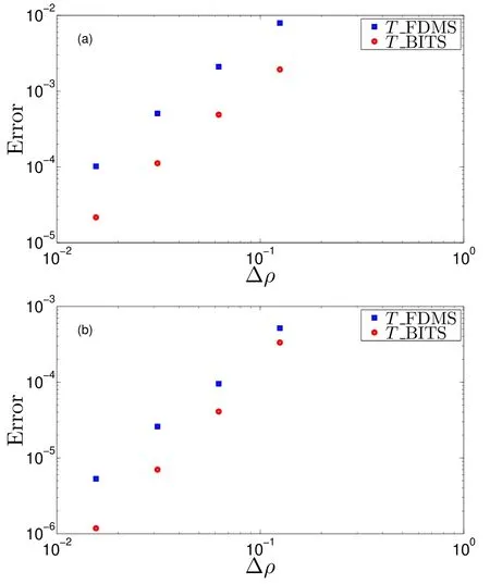
Figure 2. The error by BITS is about 1/4 to 1/5 of the error by FDMS for dt=10-2 as shown in (a).For dt=10-4,the error by BITS is still about 1/4 to 1/5 of the error by FDMS for grid points N=33,65 as shown in (b).

The errors of other cases are calculated in a similar way.They are plotted at figure 2(a).The error of temperature by BITS is about 1/4-1/5 of that by FDMS.In order to reduce the influence of time discretization,this case is recalculated using a much smaller time step(dt decreases from 10-2to 10-4),the result is plotted at figure 2(b).It is shown that the error by BITS is still about 1/4-1/5 of the error by FDMS for grid pointsN=33,65.

3.2.2.Stiff model.A stiff transport model is used to compare the performances of FDMS and BITS.

The evolution of temperatureT(ρ,t) is calculated by FDMS and BITS.The temperature profiles at the final time step by FDMS and BITS both converge as the number of grid points increases.TheN=129 results are taken as standard,and the errors of other cases are calculated as in the previous model.They are plotted in figure 3(a).The profile of χ at the last time step by FDMS and BITS is plotted in figure 3(b).The error by BITS is almost the same as by FDMS.In order to decrease the error from time discretization,the case is recalculated using a much smaller time step (dtdecreases from 10-2to 10-4).As shown in figure 3(c),the error of temperature by BITS decreases to about 1/4 to 1/5 of the error by FDMS for grid pointsN=33,65.

3.2.3.Collision model.Collisional transport is common in tokamak plasmas.The coefficients of conductivity have been computed for completely ionized gases by [28].The collisional transport coefficient varies asT-1/2.Here the transport coefficient is simplified as below:

The evolution of temperatureT(ρ,t) is calculated by FDMS and BITS.The temperature profiles at the final time step by FDMS and BITS both converge as the number of grid points increases.TheN=129 results are taken as standard,and the errors of other cases are calculated as in the previous model.They are plotted in figure 4(a).The error by FDMS is a little better than by BITS at about 0.55-0.65 of BITS.In order to decrease the error from time discretization,the case is also recalculated using a much smaller time step(dtdecreases from 10-3to 10-5).As shown in figure 4(b),the error of temperature by BITS is almost the same as the error by FDMS.

3.3.Multi-variable transport equations

In this subsection,the one-dimensional diffusion equations of densityn,electron and ion temperatureTeandTi,and the poloidal magnetic fieldBpare solved by these two methods.For simplicity,a low-β circular cross section plasma is considered,which means the geometry factors that appear at the surface average can be set as one.The equations ofn,Te,Ti,andBpare listed below:

Figure 3.The error by BITS is the same as FDMS for dt=10-2 as shown in (a).The χ at the last time step is shown in (b).For dt=10-4,the error by BITS is about 1/4 to 1/5 of the error by FDMS for grid points N=33,65 as shown in (c).

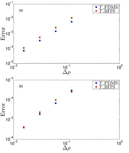
Figure 4.The error by FDMS is about 0.55-0.65 of BITS for dt=10-3 as shown in (a).For dt=10-5,the error by BITS is almost the same as the error by FDMS as shown in (b).

in whichMDBρis obtained by expanding all the elements ofMBρin equation (3) to a 4×4 diagonal matrix,

is obtained by expanding all the elements ofin equation (3) to a vector,

The derivative of variables is handled in a similar way.Then these four transport equations can be discretized into sparse linear systems and solved efficiently,just as we have done for the single transport equation case in the previous subsection.

The initial density,electron and ion temperature,and flux averaged toroidal current are set as below:

The initial poloidal magnetic fieldBpcan be integrated from the flux averaged toroidal current as below:

Then these four equation are solved by FDMS and BITS,using the predictor-corrector iteration with dt=0.001 s,100 steps.The magnetic equilibrium is fixed for simplicity.The error tolerance in iteration control is set roughly as 10-2,and only one corrector sub-step is needed for both FDMS and BITS.

TheN=129 results are taken as standard,and the errors of densityn,electron temperatureTe,ion temperatureTi,multiplication of minor radius and poloidal magnetic field ρBpare calculated as for the previous model.They are plotted in figure 5.The error of density by FDMS is about 0.6 of BITS for theN=9 case.However,the performance of BITS is improved faster as the grid points increase.The error of density by BITS is about 1/2 that of FDMS forN=65 case.The errors ofTeandTiby BITS are slightly smaller than the FDMS results for theN=9 case.The performance of BITS is improved much faster than that of FDMS as the grid points increase.The error of temperature by BITS is about 1/5 that of FDMS for theN=33 case and about 1/10 that of FDMS for theN=65 case.This means the improvement of results in FDMS by increasing the grid points is deteriorated due to the coupling of transport equations.The density equation is weakly coupled to theTeequation,and the error of density by FDMS is slightly deteriorated.TeandTihave much strong coupling with each other,and the errors ofTeandTiby FDMS are heavily deteriorated.The improvement of results in BITS by increasing grid points is still as good as in the single transport equation case (the slope ofTe,Tiby BITS is as steep as the slope of density by FDMS).The diffusion coefficient of ρBpis set as independent of others,and much smaller than the density and thermal diffusion coefficients,so ρBpvaries much more slowly.The error of ρBpby FDMS and BITS is very close for all the different grid points.

Figure 5.Error of n, Te, Ti,ρBp at the final time step by FDMS and BITS.

4.Summary

BITS is developed to solve 1-D diffusion equations for tokamak plasma based on the B-spline collocation method.It takes the same level of computation cost compared to the FDM which is widely used in existing tokamak transport codes.

The numerical results of a few cases are compared with the same order accuracy FDMS.The error of temperature by BITS is about 1/4 to 1/5 that of FDMS for the steady-state temperature transport equation case,in which no time discretization error or iteration error appears.For the singlevariable transport equation,three different transport models are used.For the simple transport model (constant χ),the error by BITS is also about 1/4 to 1/5 that of FDMS.For the stiff and collision models,the performance of BITS becomes the same or even a little worse than that of FDMS.By using a smaller time step,the error by BITS decreases to 1/4 to 1/5 that of FDMS in the stiff case or about the same in the collision case.For coupled multi-variable transport equations(collisional transport coefficients are used),the error of variables by BITS is about the same as that of FDMS,if the variable (such as density or poloidal magnetic field) is not closely coupled with other unknown variables,while the error of variables by BITS is much smaller than FDMS,if the variables (such as electron and ion temperature) are strongly coupled with each other.The improvement in FDMS results by increasing grid points is deteriorated if they are strongly coupled with each other.The improvements in BITS results by increasing grid points are still as good as in the single transport equation case.Taking the coupled 1-D tokamak plasmas transport equations as an example,the maximum errors ofn,Te,Ti,and ρBpby BITS usingN=33 are still about half of the maximum ones by FDMS usingN=65.This means BITS can reduce the computation cost by half(the computation cost of band diagonal linear equations is proportional to the number of grid pointsN),double the calculation speed and get more accurate results than FDMS.Since large computational resources are demanded when the theory-based turbulent transport model for tokamak plasmas is coupled to the 1-D transport solver to predict the time evolution of tokamak plasmas or its steady-state solution,the transport solver presented here can speed up the numerical analysis greatly.

Acknowledgments

This work was supported by the National MCF Energy R&D Program of China (No.2019YFE03040004),the Comprehensive Research Facility for Fusion Technology Program of China(No.2018-000052-73-01-001228),and the National MCF Energy R&D Program of China (No.2019YFE03060000).

Appendix

The B-spline basis function can be stably calculated by the following recurrence relation.

The first and second derivatives are listed below fork=3,tl≤x＜tl+1:

Figure A1.B(x).

In order to give a vivid picture of the basis functionB(x),let us specify a knot sequence ast1=1,…,ti=i,…,tn=n.Then for a givenxwhich falls into the intervalti≤x＜ti+1,the relevantk≤3 order basis function will take the form as below.

Bi,1,Bi-1,2,Bi,2,Bi-2,3,Bi-1,3,Bi,3have nonzero values in the interval [ti,ti+1),which are plotted in figure A1.