
Analytical model for predicting time-dependent lateral deformation of geosynthetics-reinforced soil walls with modular block facing
2024-02-29 14:50LuqiangDingChengzhiXiaoFeilongCui
Luqiang Ding,Chengzhi Xiao,Feilong Cui
School of Civil and Transportation Engineering,Hebei University of Technology,Tianjin,300401,China
Keywords:Geosynthetics Creep behavior Geosynthetics-reinforced soil (GRS) walls Lateral deformation Analytical model
ABSTRACT To date,few models are available in the literature to consider the creep behavior of geosynthetics when predicting the lateral deformation(δ)of geosynthetics-reinforced soil(GRS)retaining walls.In this study,a general hyperbolic creep model was first introduced to describe the long-term deformation of geosynthetics,which is a function of elapsed time and two empirical parameters a and b.The conventional creep tests with three different tensile loads(Pr)were conducted on two uniaxial geogrids to determine their creep behavior,as well as the a-Pr and b-Pr relationships.The test results show that increasing Pr accelerates the development of creep deformation for both geogrids.Meanwhile,a and b respectively show exponential and negatively linear relationships with Pr,which were confirmed by abundant experimental data available in other studies.Based on the above creep model and relationships,an accurate and reliable analytical model was then proposed for predicting the time-dependent δ of GRS walls with modular block facing,which was further validated using a relevant numerical investigation from the previous literature.Performance evaluation and comparison of the proposed model with six available prediction models were performed.Then a parametric study was carried out to evaluate the effects of wall height,vertical spacing of geogrids,unit weight and internal friction angle of backfills,and factor of safety against pullout on δ at the end of construction and 5 years afterwards.The findings show that the creep effect not only promotes δ but also raises the elevation of the maximum δ along the wall height.Finally,the limitations and application prospects of the proposed model were discussed and analyzed.
1.Introduction
Geosynthetics,typically made of macromolecule polymers,have been widely used in geotechnical engineering such as geosynthetics-reinforced soil(GRS)retaining walls and slopes(Han and Leshchinsky,2006;Fujita et al.,2008;Han and Jiang,2013;Xiao et al.,2022;Ding et al.,2023a).It is well-accepted that geosynthetics subjected to long-term constant static loads have significant creep behavior,as shown in Fig.1 (Zhou and Li,2011).For the non-attenuation creep curve,the total strain of geosynthetics consists of the initial elastic strain ε0and creep strain εc,which notably varies with the elapsed time,especially in the primary and tertiary stages.However,in practice,the working tensile stress of geosynthetics is often less than or equal to the allowable tensile strength(Guo et al.,2005),which is calculated using their ultimate tensile strength divided by several reduction factors to consider the effects of installation damage,creep,chemical degradation,biological degradation,etc.A smaller tensile strain can be expected at such working conditions compared to that at the ultimate tensile strength.Hence,the creep deformation of geosynthetics during operation primarily follows the attenuation creep curve,which would become stable after a certain elapsed time.

Fig.1.Typical creep behavior of geosynthetics (Zhou and Li,2011).
The lateral deformation has attracted more attention in evaluating the service performance of GRS walls as compared to equal magnitudes of vertical movement since it can cause more severe and widespread problems (Khosrojerdi et al.,2017).Liu and Ling(2007,2009) pointed out that the lateral deformation of the GRS wall would gradually increase for a long time after construction,which is caused by the creep of the backfills and reinforcements.Siddiquee et al.(2015)simulated the creep deformation of the GRS walls considering the creep rate-dependent behaviors of backfills and reinforcements.Karpurapu and Bathurst (1995) and Kazimierowicz-Frankowska (2003) found that the lateral deformation of GRS walls resulting from the creep of geosynthetics is significant.Zou et al.(2016) investigated the effect of the creep deformation of geogrids on the lateral deformation of GRS walls by numerical modeling and found that the maximum lateral deformation increases with the elapsed time.Bathurst et al.(2002)predicted the wall face deformation with a short elapsed time by integrating reinforcement strain.In short,the creep behavior of geosynthetics would cause additional lateral deformation of GRS walls(Chao et al.,2011;Allen and Bathurst,2014;Won et al.,2016).
To date,many models have been developed to predict the lateral deformation of GRS walls(Khosrojerdi et al.,2017;Kazimierowicz-Frankowska and Kulczykowski,2021),such as the FHWA method(Christopher et al.,1990),the Geoservices method (Giroud,1989),the Colorado Transportation Institute(CTI)method(Wu,1994),the Jewell-Milligan method (Jewell and Milligan,1989),and the Wu method(Wu et al.,2013).Nonetheless,these models do not involve the creep behavior of geosynthetics and thus are appropriate for GRS walls just at the end of construction (EOC).
The conventional creep tests of geosynthetics are timeconsuming and expensive,developing reliable creep models is thus critical to obtaining the actual lateral deformation of GRS walls.So far,some models have been developed to predict the creep deformation of geosynthetics under long-term loading conditions(Sawicki,1998;Sawicki and Kazimierowicz-Frankowska,2002;Zhou and Li,2011).For instance,the elasto-visco-plastic model was proposed to simulate the time-dependent behavior of geosynthetics (Peng et al.,2010;Wenzheng and Fangle,2015).TheKstiffness models were developed to investigate the mechanical behavior of the reinforcements with the elapsed time (Allen and Bathurst,2014;Yu et al.,2016a,b,2017).Allen and Bathurst(2019) developed an equation to estimate the reinforcement creep stiffness in the mechanically stabilized earth (MSE) wall design.Besides,several rheological models are also available to predict both creep deformation and stress relaxation of geosynthetics (Dechasakulsom,2001;Jeon et al.,2008;Chantachot et al.,2018;Nuntapanich et al.,2018).These various models include the relationships of material properties,stress,stiffness,and strain with the elapsed time.Although they have been proven to be effective for predicting long-term creep deformation of geosynthetics,quite a number of them are rather complicated due to many uncertain model parameters.
As discussed in Fig.1,geosynthetics under the working condition are inclined to abide by the attenuation creep curve.Therefore,an empirical hyperbolic creep model with two parameters (Zhou and Li,2011) is more popular for predicting the creep deformation of geosynthetics due to its simplicity and reliability,as shown in Eq.(1).
where ε(t)is the total strain att,εc(t)is the creep strain att,tis the elapsed time,andaandbare the fitting parameters.It is noted thatais the reciprocal of the initial slope of creep curves,whent→0,a=1/(dε/dt);bis the reciprocal of asymptotic creep strain of geosynthetics,whent→+∞,b=1/ε(t).Both of them are closely dependent on the material properties of geosynthetics and applied tensile load (Pr) levels.On the whole,ε first increases quickly and then tends to be constant witht,which conforms to the development of attenuation creep.This means that if appropriateaandbvalues are determined,the hyperbolic creep model has the ability to describe the creep behavior of geosynthetics and the resultant lateral deformation of GRS walls.
This paper first carried out a series of creep tests on two uniaxial geogrids to provide reliable data for determining thea-Prandb-Prrelationships,which were also confirmed by other experimental data from existing studies.These obtained relationships were then adopted to develop an analytical model for predicting the timedependent lateral deformation of GRS walls with modular block facing,which was further validated with the help of a relevant numerical investigation from the previous literature.Performance evaluation and comparison of the developed model with six commonly used models were performed.A parametric study was carried out to explore the effects of wall height,vertical spacing of geogrids,unit weight and internal friction angle of backfills,and factor of safety against pullout on the lateral deformation of the GRS walls at the EOC and 5 years afterwards.Finally,the limitations and application prospects of the proposed model were discussed.
2.Experimental investigation on the creep behavior of geogrids
2.1.Conventional creep tests
The conventional creep tests were carried out in this study to investigate the creep behavior of two uniaxial geogrids termed EG65R and EG90R.The geogrids are made of high-density polyethylene(HDPE)and have a quadrilateral mesh aperture with a size of 300 mm × 20 mm.Although the nominal ultimate tensile strength (Rult) of the as-received geogrids provided by the manufacturer is 65 kN/m for EG65R and 90 kN/m for EG90R,the measured ones show somewhat differences and are 64.5 kN/m and 88 kN/m,respectively referring to the ASTM D6637-11 (2011)guideline.More detailed physico-mechanical properties of the geogrids are tabulated in Table 1.The reasons for choosing EG65R and EG90R are that (i) HDPE geogrids are often encountered in practice and more prone to creep during operation(Lothspeich and Thornton,2000) and (ii) the typical tensile strength of geogrids used in field walls varies from 30 kN/m to 210 kN/m (Koerner,2010).Based on the ISO 13431(1999)standard,each sample of the geogrids for creep tests should have at least 3 ribs in the transverse direction and be 1.5 m in length along thePrdirection.
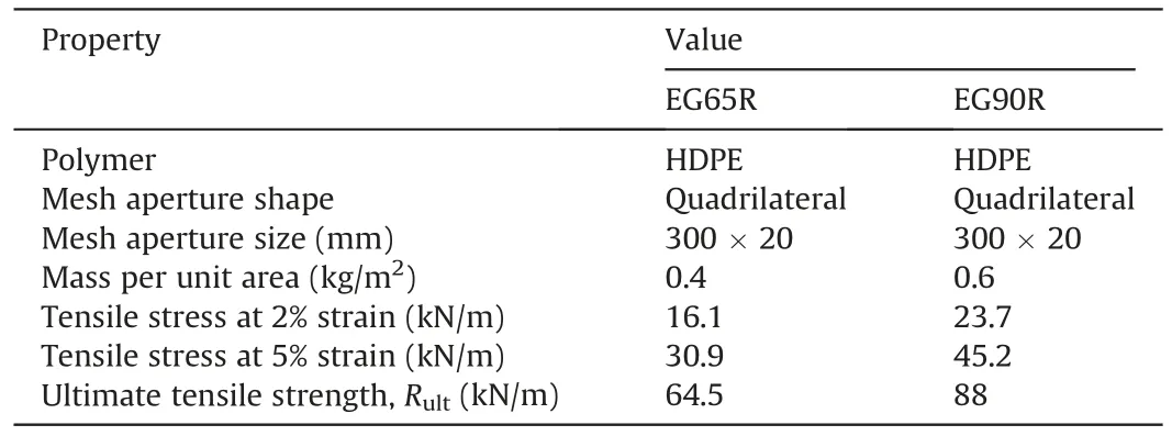
Table 1Physico-mechanical properties of the uniaxial geogrids.
Fig.2 shows the custom-made apparatus for creep tests,along with the enlarged images of two parts enclosed by red ovals.The clamping system includes a pair of steel bars with bolts and nuts,which can provide sufficient clamping power for preventing the slippage of the samples during testing.The applied tensile load per unit width of each sample is defined asPr=(TDr)/Nr,whereT,DrandNrare the applied total tensile load,the number of ribs per unit width of each sample,and the total number of ribs for each sample,respectively.Herein,DrandNrare 48.94 ribs/m and 3 ribs,respectively.Three different sustained load levels(i.e.40%Rult,50%Rultand 60%Rultfor EG65R;50%Rult,55%Rultand 60%Rultfor EG90R)were applied on the samples to determine their creep behavior in a laboratory where the temperature was maintained at 20°C (ISO 13431,1999).

Fig.2.Custom-made apparatus for creep tests: (a) Schematic diagram and (b) On-site photo.
The elongation or creep strain of the geogrids induced by variousPrlevels was determined by measuring the variation in the axial distance between the two clamps using displacement gauges.The average reading from the displacement gauges was regarded as the datum for future comparison and analysis.The testing duration was not less than 1000 h and the time intervals for recording the reinforcement strains after applying each level of load included three stages:(a)1,2,4,8,12,30 and 60 min;(b)2,4,8 and 24 h;(c)3,7,14,21 and 42 d as per ISO 13431 (1999) standard.
2.2.Analysis of testing results
Fig.3 shows the creep curves of EG65R and EG90R at three differentPrlevels.Most of the strain (ε) values for both geogrids increase rapidly at the beginning of the tests but then become constant after 100 h.In Fig.3a,the ε values at higherPrsuch as 60%Rultare much larger than those induced by lowerPrat a given time.Similar phenomena were also found in Fig.3b.In addition,the total ε is composed of ε0and εc(Fig.1).For example,corresponding toPr=40%Rult,50%Rultand 60%Rult,the creep curves of EG65R reach equilibrium at ε of 7.92%,8.92%and 13.7%.The ε0and εcvalues are 3%and 4.92%,3.6%and 5.32%,and 4.51%and 9.19%,respectively.In conclusion,the magnitude ofPrhas a significant effect on the creep behavior of both geogrids with two characteristics:higherPrcould(i)result in larger final ε and(ii)introduce a greater change rate to ε.

Fig.3.Variations in ε with t for (a) EG65R and (b) EG90R.
Fig.4 presents the isochronous creep curves and stress relaxation curves for EG65R and EG90R.These isochrones were plotted at four differenttlevels including 1 min,1 h,8 h and 72 h afterPrwas applied.All isochronous creep curves illustrate an increasing trend witht(Fig.4a).The curves for 1 h,8 h and 72 h are close as compared to the one at 1 min,which demonstrates that the shortterm ε is much larger than the ones with a longer elapsed time.Similar characteristics of isochronous creep curves were also observed in the creep tests of the HDPE geogrids reported by Dechasakulsom(2001).In Fig.4b,Prdecreases significantly within the first 100 h and then becomes flat.The smaller the given strain of geogrids is,the shorter the time duration of stress relaxation is.For example,the duration for the tensile load of EG65R decreasing from 38.7 kN/m (60%Rult) to 25.8 kN/m (40%Rult) at ε=7% is only 10 h.Nevertheless,the duration increases to about 1000 h at ε=7.9%.It demonstrates that larger strain can reduce the stress relaxation rate of the geogrids.3

Fig.4.(a) Isochronous creep curves and (b) stress relaxation curves for both geogrids.
As described above,the creep behavior of the HDPE geogrids mainly occurs within the primary and secondary stages when a low-levelPr(i.e.≤60%Rult)is applied.It means that the creep in the tertiary stage typically follows the rupture of geogrids,which does not occur to both EG65R and EG90R since the adoptedPris not large enough.Dechasakulsom(2001)conducted a series of creep tests on HDPE geogrids subjected to 30%,40%,60% and 80% ofRult,and found that whenPrincreases up to 80%Rult,ε develops faster and then the rupture scenario occurs within 200 min.Whereas,the geogrids reach a constant ε after several days when thePrlevels are 30%Rultand 40%Rult.In a word,ε develops progressively whenPris small,such as less than 60%Rultdue to the effects of several reduction factors as mentioned earlier.Hence,the creep development of geogrids in field GRS walls could last for a long time after construction.
2.3.Determining the relationships of parameters a and b with Pr
The creep data of EG65R and EG90R shown in Fig.3 were predicted using Eq.(1).Fig.5 compares the measured creep values(in symbol) with the predicted ones (in line),along with the corresponding coefficient of determination (R2).The measured data are distributed on or near the predicted lines.The fact ofR2≥0.98 demonstrates that Eq.(1)is effective to describe the creep behavior of both tested geogrids.
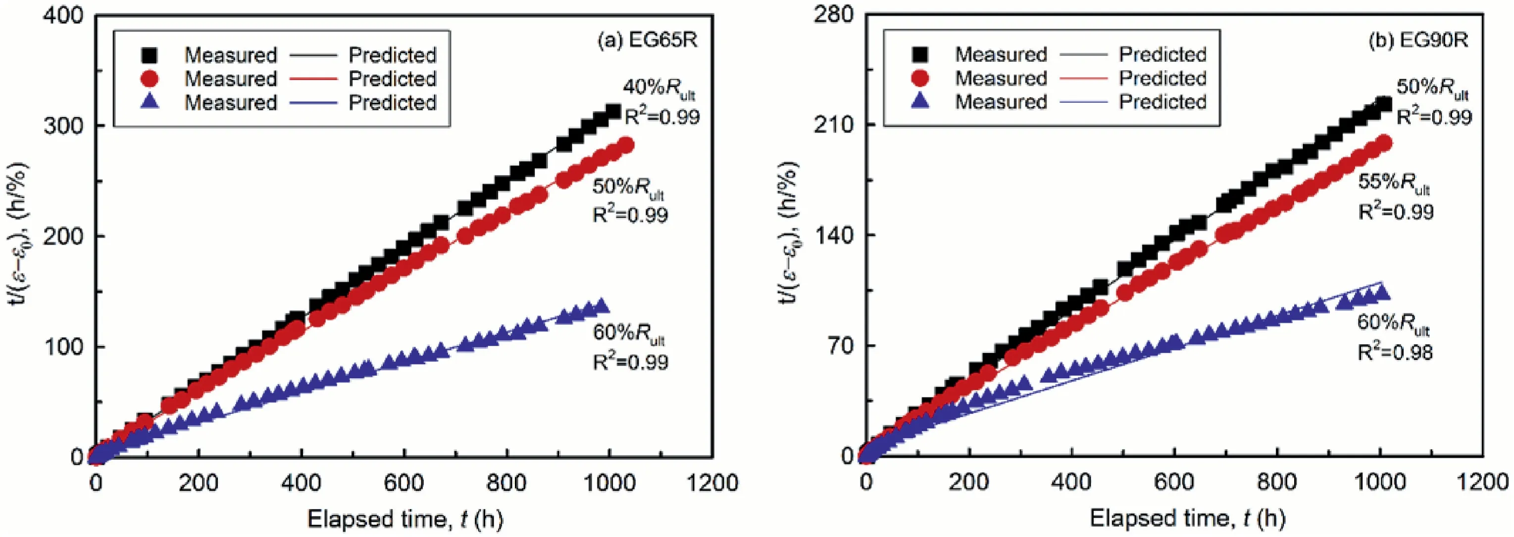
Fig.5.Comparisons between the measured and predicted creep values using Eq.(1): (a) EG65R and (b) EG90R.
Note that using two HDPE geogrids experiencing 40%Rult-60%Rultto determine the relationships of parametersaandbin Eq.(1)withPris limited since they are related to the type of geosynthetics andPrlevels(França et al.,2013;Filho et al.,2019).Additional creep data of different geosynthetics under variousPrlevels (5%Rult-60%Rult) were therefore collected from existing literature.These geosynthetics include geogrids and geotextiles made of HDPE,polyethylene-terephthalate (PET),polypropylene (PP),polyester(PE),or PP and PE (PP-PE).In total,18 geosynthetics were used to establish the relationships ofavs.Prandbvs.Pr,as summarized in Table 2.Apparently,agrows exponentially withPrwhile theb-Prrelationship demonstrates a negative linear correlation(R2≥0.85).In the following section,the obtaineda-Prandb-Prrelationships were adopted to develop an analytical model for predicting the time-dependent lateral deformation of GRS walls considering such creep effect.

Table 2Relationships of a and b with Pr obtained from existing literature and this study.
3.Development of analytical model for predicting the lateral deformation of GRS walls
Compared with conventional cantilever and gravity retaining walls,GRS walls with flexible facing generally have relatively larger lateral deformation.The commonly used model for the design of GRS walls is the Jewell-Milligan method(Jewell and Milligan,1989)owing to its simplicity,in which the rigidity of wall facings and the creep behavior of reinforcements are neglected.Although Wu et al.(2013) have improved the Jewell-Milligan method by considering the friction between adjacent facing blocks to calculate the lateral deformation of modular block GRS walls,the creep behavior of reinforcements has gained little attention in the Wu method (Wu et al.,2013),as well as other methods (Giroud,1989;Christopher et al.,1990;Wu,1994).Therefore,relevant methods reflecting the creep effect are still scarce.
Jewell and Milligan(1989)assumed that the lateral deformation of GRS walls with enough long reinforcement is mainly caused by the reinforcement in Zone-1 and Zone-2,as shown in Fig.6a.According to the force equilibrium principle,the tensile force of reinforcements in the active zone(i.e.Zone-1)should be equal to the pullout resistance of reinforcements in the stable zone.Thus,the effective length,Lei,of reinforcements in the stable zone shown in Fig.6b,which can be calculated using the force equilibrium principle,is probably smaller than the effective length (i.e.LZone-2i) of reinforcements recommended by the Jewell-Milligan method.That is,theLZone-2ivalue can be overestimated if the Jewell-Milligan method is followed in practice.Thereby,an analytical model was proposed here to overcome such drawbacks and the detailed procedures for developing this model are as follows.
3.1.Basic assumptions
Similar to the Jewell-Milligan method,the assumptions used for establishing the analytical model are also in connection with the tensile force distribution of reinforcements in both active and stable zones and the potential failure surface of GRS walls.Specific assumptions are described below:
(1) GRS walls with vertical modular block facing and equally spaced reinforcements are constructed on rigid foundations.The reinforcement length is sufficient for the walls’ internal stability.
(2) The lateral deformation of the walls only results from the deformation of reinforcements,consisting of elastic and creep elongations.
(3) The potential failure surface inside GRS walls conforms to the Rankine failure surface,which is typically formed with an inclination angle of 45°+φ/2 to the horizontal,where φ is the internal friction angle of backfill materials (Fig.6b).
(4) External surcharges from dynamic traffic loads acting on the top surface of GRS walls are regarded as uniformly distributed loads.
(5) The tensile force is evenly distributed in the reinforcement in the active zone but shows a linearly decreasing trend in the stable zone.Note that the tensile force in the stable zone only exists withinLeithat can be determined by the pullout resistance of reinforcements,beyond which the tensile force is equal to zero (Fig.6b).This assumption is different from the Jewell-Milligan method,in whichLeiis equivalent toLZone-2idetermined by the horizontal distance between the potential failure surface and the repose φ plane,as shown in Fig.6a.
3.2.Elastic deformation of reinforcements
After the construction of GRS walls,the instant elastic deformation of reinforcements immediately occurs due to the lateral earth pressure.In Fig.6b,theith reinforcement length with tensile forceLiconsists ofLai(i.e.the length in the active zone) andLei,which can be calculated respectively by the geometrical relationship and force equilibrium (Elias et al.,2001):
whereziis the depth of theith reinforcement layer below the crest of the walls;FSpis the factor of safety against pullout(typically 1.5-2);Prmiis the maximum tensile load per unit width of theith reinforcement layer;Cis surface area geometry factor and equals 2 for strip,grid and sheet type reinforcements;Rcis the coverage ratio and defined asb′/Sh,in whichb′is the gross width of a reinforcement element andShis the center-to-center horizontal spacing between adjacent reinforcement elements;F* is the pullout resistance factor and can be taken conservatively as 2/3tanφ(28°≤φ ≤34°);α is the scale correction factor,0.8 for geogrids and 0.6 for geotextiles;and σviis the vertical stress at theith soilreinforcement interface.FHWA (2009) suggested that when each reinforcement layer covers the entire horizontal surface of the reinforced soil zone (i.e.continuous reinforcement),the values ofSh,b′,and resultantRcshould be 1.
Based on Assumptions (3)and (4),the horizontal stress behind the wall facing at theith soil-reinforcement interface can be calculated as
whereKais the Rankine active earth pressure coefficient;σhiis the horizontal stress at theith soil-reinforcement interface;γ is the unit weight of backfill materials;andqis the equivalent welldistributed load induced by overlying surcharges.The tensile force distribution along theith reinforcement layer is written by
wherePri(x) is the tensile load atx;Svis the center-to-center vertical spacing between adjacent reinforcement elements;andxis the horizontal distance to the back of the wall facing.
At theith layer,the elastic deformation dδeiof reinforcements within a length of dxcan be expressed as
where ε0iindicates ε0of theith reinforcement layer,andKreinfis the reinforcement stiffness.Integrating Eq.(5),the elastic deformation or elongation δeiat theith reinforcement layer in both active and stable zones can be given by
Substituting Eqs.(2b),(2c)and(3)and(4)into Eq.(6),we have
WhenRcequals 1,Eq.(7) can be simplified as
3.3.Creep deformation of reinforcements
The creep strain of reinforcements in a period of dtis equal to dεc(t),as shown in Fig.1.The creep deformation dδciof theith reinforcement layer with a length of dxcan be known as
Taking the derivative of the term dεci(t)with the aid of Eq.(1),it can be determined as
Substituting Eq.(10)into Eq.(9)and then integrating Eq.(9),the creep deformation δciof theith reinforcement layer can be identified as
The total deformation δiof theith reinforcement layer is the sum of δeiand δci,as described in Eq.(12).It also represents the creep effect-induced lateral deformation of GRS walls according to Assumption (2).
In conclusion,the following parameters regarding GRS walls should be determined before using Eq.(12) to predict the timedependent lateral deformation δ:
(1) Geometric quantities: wall height (H),reinforcement length(L),center-to-center vertical (Sv) and horizontal (Sh)spacing between adjacent reinforcement elements,depth of theith reinforcement layer (zi);
(2) Material characteristics:unit weight(γ)and internal friction angle(φ)of backfill materials,reinforcement stiffness(Kreinf),a-Prandb-Prrelationships of reinforcements;
(3) External surcharges: equivalent well-distributed loads (q);
(4) Other parameters: factor of safety against pullout (FSp),pullout resistance factor (F*),scale correction factor (α),surface area geometry factor(C),coverage ratio(Rc),elapsed time (t).
These parameters are fundamental and significant for engineers and technicians when designing and analyzing GRS walls with modular block facing in a field.What may matter more is the ease of their availability either directly or indirectly.This manifests that the proposed analytical model is simple and straightforward in terms of its application.
4.Validation,evaluation and comparison of the proposed model
4.1.Performance validation and evaluation
Existing studies mainly focus on either the lateral deformation of GRS walls at the EOC or the creep behavior of geosynthetics,which makes it hard to obtain all validation data at once in physical and field test examples.Therefore,only a previous numerical investigation performed by Liu et al.(2009) on the long-term behavior of GRS walls considering reinforcement creep was adopted here to validate the proposed model.The corresponding schematic diagram of the GRS numerical model wall is presented in Fig.7.The model wall with a heightHof 8 m was constructed on a dense sandy foundation overlying the rigid rock base.The used backfill soil is 20 kN/m3in γ and 30°in φ.Thirteen layers of geogrids termed Grid A withSv=0.6 m andSh=0 m were used as the reinforcement,whose length is 0.7H=5.6 m larger than the maximum value of(H-0.6)tanφ=4.3 m.More detailed descriptions of the numerical model wall can be found in Liu et al.(2009).
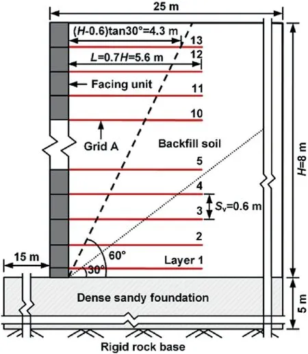
Fig.7.The GRS numerical model wall modified from Liu et al.(2009).
Fig.8 shows the experimental and numericalPr-ε relationships for Grid A and EG65R.ThePrvalues of both geogrids exhibit minor differences of 0.1 kN/m at ε=2% and 2.4 kN/m at ε=5% between the experimental results and of 2.2 kN/m at ε=2%and 2.9 kN/m at ε=5% between the experimental and numerical results.This means that both geogrids have almost identical stiffness properties such asKreinf.Therefore,theKreinfvalue of EG65R was deemed to be that of Grid A (i.e.1300 kN/m).

Fig.8.The Pr-ε relationships of Grid A and EG65R.
The creep curve of Grid A atPr=6 kN/m was available in Liu et al.(2009) (Fig.9).To illustrate the similarity of creep behavior between Grid A and EG65R,thePr-ε0relationship of EG65R was established using the measured data,which follows ε0=0.115PrwithR2=0.99.Combined with thea-Prandb-Prrelationships of EG65R shown in Table 2,ε0,aandbatPr=6 kN/m were calculated to be 0.69%,0.873 and 0.593,respectively.Substituting these values into Eq.(1),the corresponding creep curve was plotted in Fig.9.It can be seen that the creep behaviors of both geogrids are similar,especially at highertlevels.Hence,thea-Prandb-Prrelationships of EG65R are also appropriate for Grid A.In addition,there is noqacting on the top surface of the wall and the values ofFSp,C,Rc,α,F*andtare respectively 1.5,2,1,0.8,2/3tanφ=0.38,and 43,800 h(5 years),which were adopted in Eq.(12) for the subsequent model validation.

Fig.9.The Pr-ε0 relationship of EG65R and the creep curves of Grid A and EG65R at Pr=6 kN/m.
Fig.10 shows the variations inLZone-2i,LeiandLiof the numerical model wall withh,accompanied by the potential failure surface and the repose φ plane.It can be seen thatLeifrom the proposed model remains a constant of 0.5 m with increasingh.The reason can be explained by the fact that combined with Eqs.(3)and(4),Eq.(2c)for calculatingLeican be reassembled as Eq.(13).This equation indicates thatLeiis irrelevant tohand hence keeps constant for all reinforcement layers.

Fig.10.Comparison of the reinforcement lengths at each layer in the numerical model wall obtained from the Jewell-Milligan method and proposed model.
In the Jewell-Milligan method,LZone-2iof the bottommost layer is 0.2 m less than the constantLeiof 0.5 m.After that,it exceedsLeiand continues to increase at a speed ofSv[tan(90°-φ)-tan(45°-φ/2)]withh.Whenhis equal to 7.4 m,a significant difference of 8 m can be found betweenLZone-2i(8.5 m) andLei(0.5 m),leading to a 94%reduction in the reinforcement length.This fact indicates that mostLeiis indeed less thanLZone-2i,which confirms the effectiveness of Assumption(5)used in the proposed model.In addition,Liin the Jewell-Milligan method grows faster than that in the proposed model ashincreases,resulting in a significantly widening difference between them.This is associated with the magnitude relation betweenLZone-2iandLei.Eventually,Liin the Jewell-Milligan method exactly follows the repose φ plane as anticipated,while theLidata for the proposed model are distributed between the potential failure surface and the repose φ plane.
Fig.11a illustrates the numerical δnand predicted δpat the EOC and 5 years afterwards versus the normalized wall height(h/H).For all curves,δ first increases and then turns to decrease with increasingh/H.This contributes to the scenario that the maximum values occur ath/H=0.55 for δnandh/H=0.48 and 0.63 for both δp.As stated by Sabermahani et al.(2009),GRS walls during service deform typically following three modes such as bulging,overturning and sliding.Visually,the numerical model wall can be assigned to a bulging deformation mode.Such observation is consistent with the deformation behavior of the previously reported GRS walls with modular block facing suffering static footing loading (Xiao et al.,2016),dynamic vehicle loading (Ding et al.,2023b),and even destructive seismic loading (Ling et al.,2005).It indicates that although there is no external surcharge(i.e.q=0)for the wall,its deformation mode is still consistent with those of GRS walls suffering various loadings.

Fig.11.Relationships of (a) δ with h/H and (b) δn with δp.
In addition,the maximum δn(80.7 mm)and δp(93.19 mm)after 5 years respectively increase by 156% and 196% compared to the maximum δp(31.5 mm) at the EOC.Therefore,it is of great significance to consider the long-term creep effect of geosynthetics in the design of GRS walls when using the analytical model.Since the generated δnand δplarger than 1%H(80 mm)are within 0.9%H-4%H,which is the maximum δ suggested by FHWA (2009) and AASHTO(2020).
More importantly,the δpvalues after 5 years are close to the numerical ones below the middle of the wall.However,they do not match very well (i.e.overestimation) in the upper portion of the wall.The following possible reasons may be attributed to such difference:
(1) It is assumed that the tensile force in the active zone is distributed uniformly and equal to the maximum tensile force of the geogrids at the potential failure surface,which may overestimate the tensile force of the geogrids in the active zone.Consequently,the creep deformation of the geogrids and the resultant lateral deformation of the wall facing also might be overestimated.
(2) In Fig.7,the concrete facing blocks of the wall are 2 ×10⁴MPa in Young’s modulus and their interfaces follow the Mohr-Coulomb failure criterion during simulation.Yet,the rigidity of the facing was not involved in the proposed model,which contributes to the overestimation of the lateral deformation of the wall.
(3) The GRS wall was constructed on a dense sandy foundation rather than the rigid foundation.Under the action of the selfweight,the vertical deformation of the wall is probably uneven along the reinforcement elongation direction.Typically,the settlement behind the facing is smaller than that of other locations away from the facing due to the pocket effect from the reinforcement (Lu et al.,2020).Meanwhile,the compressible sandy foundation boosts such differential settlement,which lessens the wall lateral deformation.
Statistical analysis was carried out on the obtained δppredictions to determine their mean bias (MB),root mean squared error (RMSE),and coefficient of variation (COV) by means of Eqs.(14)-(16),respectively.Parametermis the number of reinforcement layers and equals 13 (Fig.7).In the statistical analysis,MB is defined as the mean ratio of δpto δn.Thus,MB<1 indicates a radical prediction model whileMB>1 represents a conservative one.RMSE and COV represent the accuracy and reliability of the proposed model,respectively.Larger values of them mean that the model is less accurate and reliable.Similar statistical analyses were also executed by Khosrojerdi et al.(2017) and Zou et al.(2021) on the evaluation and comparison of performance for the prediction models developed in their studies and other previous literature.
Fig.11b describes the relationship of δpwith δnbased on the data after 5 years shown in Fig.11a,along with the MB,RMSE and COV values.All data are located above line 1:1 where δpis the same as δn,showing the overestimation scenario.The MB value of 1.1 indicates the proposed model is somewhat conservative.Even so,RMSE=9.56 andCOV=0.31 are still situated at lower levels(Khosrojerdi et al.,2017;Zou et al.,2021),confirming that the model is accurate and reliable.Overall,the proposed model is effective to predict the time-dependent lateral deformation of GRS walls considering the creep effect of geogrids.
4.2.Performance comparison
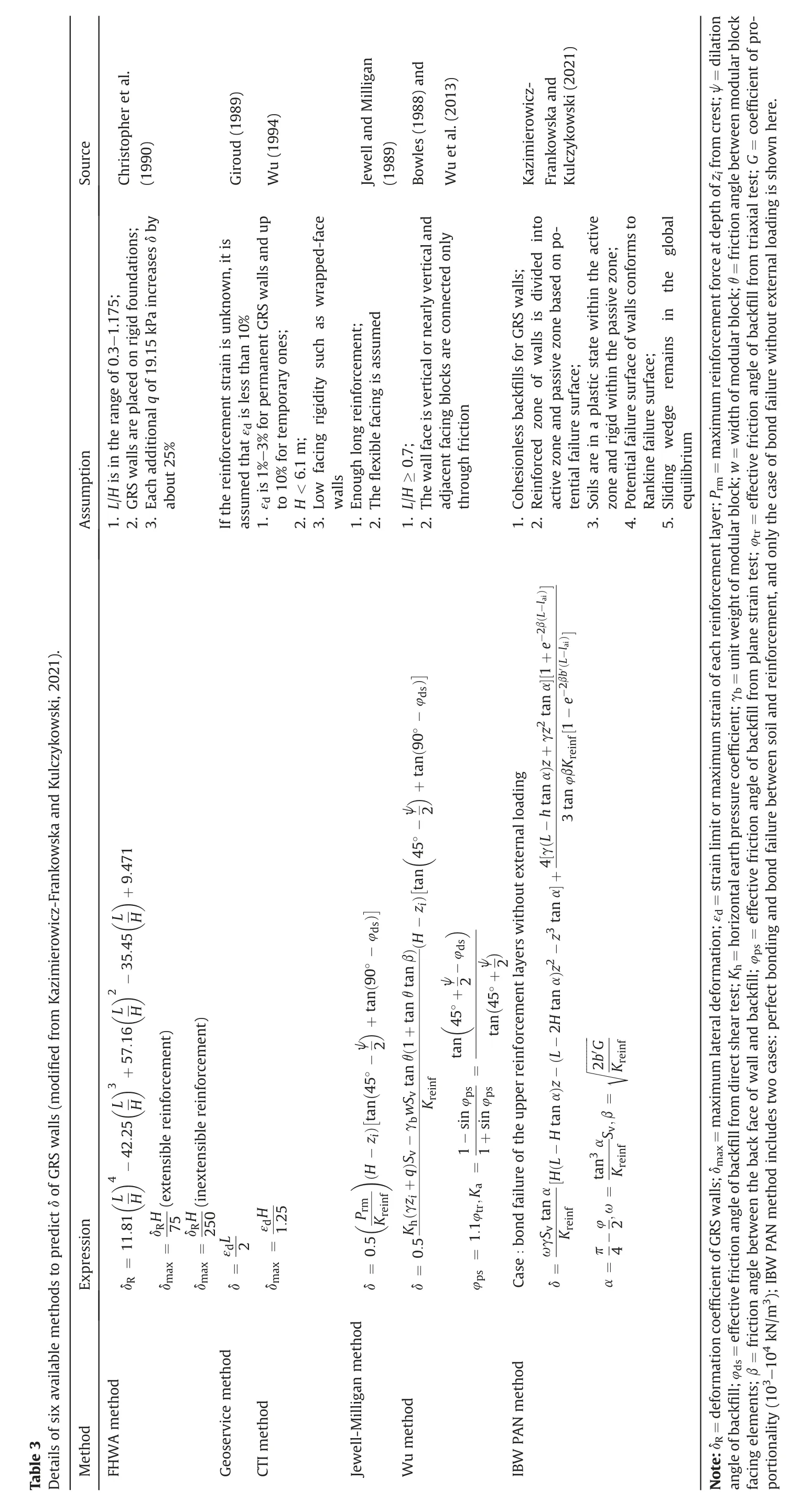
Table 3 lists six available methods to predict δ at the EOC,including five classical methods and one recently developed IBW PAN method.Although the first five are a little old,it does not represent that all of them are conservative (Khosrojerdi et al.,2017).Furthermore,Kazimierowicz-Frankowska and Kulczykowski (2021),taking the five classical methods as reference levels,have proved the accuracy of the IBW PAN method with success.For achieving a step forward,the six methods were adopted here to provide predictions of the numerical results described in Fig.11 for evaluating the proposed model as thoroughly as possible.
Fig.12 presents the comparison between the numerical and predicted δmaxusing the six methods and the proposed model.The δmaxvalues determined by the CTI method,Jewell-Milligan method,Wu method,and IBW PAN method are below the full line where the numerical δmaxis equal to 80.7 mm.This means that the four methods underestimate δmaxdue to having no consideration of the creep of geogrids,and hence are somewhat radical.The FHWA method and Geoservice method also did not involve the creep effect,they however are conservative.The reason is that the FHWA method(i)was developed based on regression analysis of abundant data collected from actual GRS structures and numerical simulations,whose design and construction conditions are probably not the same as those used in Liu et al.(2009),and(ii)relies too much on the geometry of GRS walls and abutments,which is generally not as accurate as those that take backfill mechanical properties,reinforcement strain or force as variables.The Geoservice method provides the most conservative prediction based on the mean εd=5%since the reinforcement strains for all layers were unknown in Liu et al.(2009).

Fig.12.Comparison between the numerical and predicted δmax using the six methods and the proposed model.
The closest distance (11.6 mm) between the full line and predictions was observed in the IBW PAN method rather than the proposed model (12.5 mm),which is followed by the Jewell-Milligan method (13.6 mm) and Wu method (15.6 mm).Even so,the proposed model still provides well δ predictions for the global facing compared to the above three methods.Since their predictions exhibit obviously scattered at the upper portion of the wall as shown in Fig.13a.This induces MB to decrease and RMSE and COV to increase(Fig.13b),stating that the proposed model is more accurate and reliable.
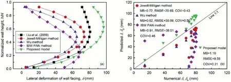
Fig.13.Comparison between the numerical and predicted δ using the available methods and the proposed model.
5.Parametric study on the lateral deformation of GRS walls
A typical GRS wall that is most often encountered in practice was introduced here for parametric analysis.The typical wall constructed on a rigid foundation is backfilled with granular soil and reinforced with EG65R.Following are the parameters selected for the wall based on the previous literature(FHWA,2009;Xiao et al;Gao et al.,2022):(i)H=6 m,L=0.7H=4.2 m,Sv=0.6 m,Sh=0 m,andzi=0.6-5.4 m (9 levels);(ii) γ=18 kN/m3,φ=34°,Kreinf=1300 kN/m,anda-Prandb-Prrelationships of EG65R (see Table 2);(iii)q=15 kPa;(iv)C=2,FSp=1.5,Rc=1,α=0.8,andF*=0.45.The reason for choosing EG65R as the reinforcement is that the working stress of geogrids is assumed to be less than 40%Rultfor ensuring the stability of GRS walls(Zou et al.,2016).In this study,the maximumPrmi(i.e.Prm1) is equal to 16.5 kN/m via a preliminary calculation,which accounts for about 26%Rultof EG65R and satisfies the needs of working stress conditions.
A parametric study was performed using the proposed model to determine the effects of several variables such asH,Sv,γ,φ andFSpon the δ response of GRS walls experiencing differenttlevels.It is reported that the growth of δ is mainly concentrated in the first 5 years after construction,demonstrated by the previous research results,i.e.δ=0.15H,0.5H,0.53Hand 0.58Hat the EOC,5 years,10 years and 15 years afterwards,respectively(Zou et al.,2016).Hence,taking the EOC and 5 years afterwards as representativet,Table 4 provides the summary of these variables and their values (FHWA,2009;Gao et al.,2022),where the bold numbers are used for the typical GRS wall (herein also referred to as a benchmark wall).In the parametric analysis,the benchmark wall evolved into different GRS walls by varying these investigated variables,i.e.one variable as well as its resultant variables(if available)changed following the assigned values and the others kept constant for each wall.Totally,48 cases including 8 duplications were involved in the parametric analysis.
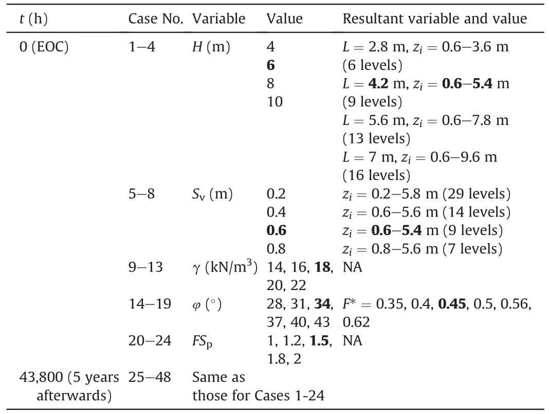
Table 4Case summary of the parametric study.
Fig.14 presents the δ-h/Hrelationships of the EG65R reinforced GRS walls with variousH,Sv,γ,φ andFSplevels at the EOC and 5 years afterwards.For each δ-h/Hcurve,the maximum δ was denoted as δEOCor δ5ausing symbols in a star fashion.This aims to highlight(i)the effect of each variable on the long-term δ response of the walls and (ii) the difference between δEOCand δ5aand their ratio relationship such as δEOC/δ5afor each variable.Detailed δEOC,δ5aand δEOC/δ5avalues for all cases are listed in Table 5.

Table 5δEOC and δ5a values and their ratio relationships for all cases.
In Fig.14a,fourHlevels vary from 6 m to 4,8 and 10 m to investigate the effect ofHon δ.Apparently,increasingHleads to a significant increase in δ,and the largerHis,the faster δ increases.To be specific,the total increase is about 5.74 times for δEOCand 2.81 times for δ5awithin the investigatedHrange (Table 5).The maximum δEOCand δ5arespectively appear in Cases 1 and 25(H=10 m) and are 33.26 mm ath/H=0.46 and 100.59 mm ath/H=0.64.The obtained δEOCnormalized byHis distributed within 0.14%-0.33%,which almost coincides with the δEOC/Hrange of 0.1%-0.3%suggested in the NNG(2004)criterion.By contrast,δ5a/His more prominent with a higher range of 0.9%-1.01% and its correspondingh/Hlevel after 5 years of service is elevated from 0.4 to 0.5 to 0.64-0.85.This is consistent with the numerical results reported in the literature (Liu et al.,2009;Zou et al.,2016).Besides,δ5ais about 6.19 times δEOCatH=4 m and this ratio reduces to 3.02 whenHis up to 10 m,despite the two individuals (δEOCand δ5a)showing an increasing trend withH.
Such phenomenon indicates that (i)Hplays a crucial role in influencing δ,especially for the middle portion of the walls at the EOC and for the upper portion of the walls at 5 years afterwards;(ii)compared to δei,δciof the geogrids dominates in the total δi,which alters the distribution mode of δ alongHin terms of amplitude and location;(iii) the relationship of δ5a/δEOCwithHis negatively correlated and opposite to those of δ5aand δEOCwithH.
The possible reason is that increasingHenhances the horizontal stress σhiin Eq.(3) and then tensile forcePri(x) in Eq.(4) of the geogrids at a givenh/Hlevel,which facilitates both δeiin Eq.(6)and δciin Eq.(11) of the geogrids and thereby δ of the GRS walls.As depicted in Figs.6 and 10,Licomposed of differentialLaiin Eq.(2b)and identicalLeiin Eq.(16) increases withh.It means that the geogrids at the upper portion of the walls produce more creep deformation after 5 years as compared to the middle ones.Hence,the initial δEOCshifts from the middle to the upper portion of the walls where the final δ5ais located.In Fig.3a,more attention has been directed to the creep behavior of the geogrids at differentPrlevels.However,it is worth noting that increasingPralso increases the initial ε0,as well as δEOC.For instance,the ε0values are 3%at 40%Rult,3.6%at 50%Rult,and 4.51%at 60%Rult.IncreasingHthus raisesPrand δEOC,inhibiting the development of δ5a/δEOC.
FHWA(2009)recommended that the maximum vertical spacing of reinforcements should not exceed 0.8 m for the safety of GRS walls.FourSvlevels including 0.2,0.4,0.6 and 0.8 m were adopted to explore the effect ofSvon δ,as shown in Fig.14b.It is evident that the closerSvgenerates the smaller δ alongH.This is due to that decreasingSvwould lead to an increase inm,which on the one hand reduces the tensile force of each reinforcement layer and on the other hand increases the rigidity of the reinforced zone.Combination of these two aspects results in smaller δ.However,it is noted that althoughSv=0.2 m represents a relatively rigid wall,the creep effect still triggers a larger δ5aof 48.01 mm (0.8%H) ath/H=0.97 as compared to δEOC=3.88 mm (0.06%H) ath/H=0.5(Table 5).More undesirably,the maximum δEOCand δ5aatSv=0.8 m are respectively 17.28 mm (0.29%H) ath/H=0.47 and 60.11 mm (1%H) ath/H=0.73.It indicates that the creep deformation of the walls becomes remarkable with increasingSv,which cannot be neglected even in the case of densely laid reinforcements.
Comparison of(max.δEOC)/δEOC≤4.45 with(max.δ5a)/δ5a≤1.25 states that δEOCof the as-constructed GRS walls is more sensitive to the variation inSv.It is attributed to the fact that the parameterSvreflects the rigidity performance of the walls.δEOCgenerally occurs at the elastic stage of the geogrids and hence shows a closer relationship with varyingSv.Due to this reason,the creep effect is weakened by increasingSv,reflected by the ratio δ5a/δEOCvarying from 12.37 to 3.48.Such a scenario is consistent with the observation from the relationship of δ5a/δEOCwithH.
To further evaluate the effect of backfill properties on δ,Fig.14c and d presents the δ-h/Hrelationships respectively at five γ levels including 14,16,18,20 and 22 kN/m3and six φ levels including 28°,31°,34°,37°,40°and 43°.Evidently,high-quality soils for backfilling GRS walls possess smaller γ such as 14 kN/m3and larger φ such as 43°since δEOCand δ5aare the smallest under such circumstances.This finding is in agreement with the φ values of 34°-40°for reinforced backfills recommended by FHWA (2009).The reason is that smaller γ and larger φ would reduce σhiand then δ.Moreover,a larger δ span between adjacent curves can be found in Fig.14d rather than in Fig.14c,indicating changing φ is more effective to restrict δ(especially for δ5a)than changing γ.This can be explained by the fact that compared to γ,the term tan(45°-φ/2)in Eq.(3) is in a quadratic form,which can magnify the effect of varying φ on δ.Hence,it is suggested that soils with edges and corners are better choices for GRS walls to eliminate the creep effect.
Fig.14e shows the δ values at fiveFSplevels including 1,1.2,1.5,1.8 and 2.All curves with differentFSpoverlap at the EOC but yield a slight distinction at 5 years afterwards,meaning that δ is less influenced by varyingFSp.In fact,FSpis only used to calculateLeiin Eq.(2c),which accounts for a small proportion ofLi(Fig.10).Thus,the change ofFSphas little influence on δ.Moreover,it is concluded from Fig.14a-e that for the GRS walls with variousH,Sv,γ,φ andFSp,the creep of the geogrids not only introduces a significant increase to δ but also elevates the location of the maximum δ.The relevant reason has been discussed earlier.
6.Discussion
In the present study,an analytical model was proposed based on the general hyperbolic creep model of geosynthetics to predict the time-dependent δ of GRS walls with modular block facing.Due to the accepted fact thatPris more less thanRult,the proposed model works in cases where geosynthetics under the working stress conditions follow the attenuation creep.However,two factors responsible for δ were still not considered in the model,and the resultant limitations are as follows:
(1) The analytical model is encouraged to be applied directly to GRS walls with less facing rigidity,which was not involved in the current study.As is well known that the facing rigidity is related to blocks’ weight,dimension,number of layers,connection mode,and so on.Heavier and thicker blocks,fewer block layers,or firmer connections between adjacent blocks could result in higher facing rigidity and therefore smaller δ.For example,heavy facing blocks could introduce a 35% reduction to the maximum δ compared to weightless blocks(Wu et al.,2013).On the other hand,an increase in the facing rigidity would probably elevate the location of the maximum δ (Vieira et al.,2008).Hence,the contribution of the facing rigidity to δ should be considered when the model is used for GRS walls with higher facing rigidity.
(2) The proposed model is more suitable for GRS walls with granular soils (low fines content) due to having no consideration of the creep of backfill materials.Typically,finegrained soils used for GRS walls would deform to some extent(i.e.creep deformation)under the long-term action of the self-weight and/or external surcharges,despite having been compacted to more than 95%of the maximum degree of compaction during construction.Such a creep scenario is attributed to the dissipation of excess pore water pressure in these soils (referred to as secondary consolidation) and becomes more obvious with increasing fines content.When the creep of the soils is larger than that of geosynthetics,it can increase the reinforcement load.On the contrary,geosynthetics experience load relaxation,leading to an increase in overall soil deformation.Anyway,the soil creep makes δ increase (Liu et al.,2009) and thus the model may underestimate it.By contrast,the creep of granular soils with low fines content induced by the secondary consolidation is indeed minimal and can be neglected.Hence,it should be cautious to use the model for estimating the long-term δ of GRS walls backfilled with fine-grained soils.
Besides,the limited data available in existing literature led to a preliminary validation,evaluation and comparison of the proposed model.Although far from exhaustive,such preliminary results are promising.Certainly,the next research is necessary to be carried out via physical model tests,which are similar to those performed in Cui et al.(2022) and Ding et al.(2023b) but focus on the longterm δ of GRS walls.Combining with the creep results of the corresponding geosynthetics,the intended research is expected to provide whole data information as mentioned in Section 3 for the further development of the proposed model.
Currently,multi-tiered GRS walls have been considered as an appropriate alternative.Therefore,a more interesting thing is that the analytical model is also expected to evolve into an advanced one,which is no longer limited to single-tiered GRS walls but focuses more on GRS walls in tiered configurations considering the combined effects of the creep of geosynthetics and offset distance(D).Unfortunately,the advanced model is not involved in this study due to the absence of validation data.In fact,Gao et al.(2022)have brought forward an analytical solution to estimate the lateral deformation behavior of two-tiered GRS walls at the EOC.Although the creep effect of geosynthetics was also not considered in the solution,it is likely to provide valuable insights into the deformation characteristics and mechanisms of two-tiered walls.This contributes to further relevant research by highlighting such combined effects.
7.Conclusions
In accordance with the force equilibrium principle,this study proposed an analytical model for predicting δ of GRS walls with modular block facing using the hyperbolic creep model of geosynthetics.Performance validation,evaluation and comparison of the proposed model were carried out,as well as the parametric analysis focusing on the effects ofH,Sv,γ,φ andFSpon δ.The following conclusions can be drawn:
(1) Both HDPE geogrids exhibit attenuation creep whenPris less than 60%Rult.The parameterain the hyperbolic creep model grows exponentially withPr,while theb-Prrelationship follows a negative linear correlation.
(2) An analytical model was proposed to predict δ considering the creep effect of geosynthetics,which was validated to be accurate and reliable.The CTI method,Jewell-Milligan method,Wu method,and IBW PAN method underestimate δmaxand hence are somewhat radical.The opposite observation was found in the FHWA method and Geoservice method.The proposed model is more accurate as compared to the above six methods.
(3) Decreasing φ or increasingH,Svand γ can accelerate the development of δ.However,the effect of varyingFSpon δ is insignificant.For all variables,the creep effect of the geogrids makes the maximum δ shift from the middle to the upper portion of the walls.This requires that designers and technicians should focus more on the upper δ of the walls during long-term operation.
(4) Special attention should be paid to GRS walls with higher facing rigidity and/or fine-grained soils when employing the proposed model to predict δ.Since the positive contribution of the wall facing rigidity and the negative contribution of the soil creep cannot be neglected.Furthermore,the proposed model is expected to evolve into the one appropriate for multi-tiered GRS walls considering the combined effects of geosynthetics creep andD.
Data availability statement
All data,models,or code that support the findings of this study are available from the corresponding author upon reasonable request.
Declaration of competing interest
The authors declare that they have no known competing financial interests or personal relationships that could have appeared to influence the work reported in this paper.
Acknowledgments
This research work was financially supported by the National Natural Science Foundation of China (Grant Nos.52078182 and 41877255) and the Tianjin Municipal Natural Science Foundation(Grant No.20JCYBJC00630).Their financial support is gratefully acknowledged.
 Journal of Rock Mechanics and Geotechnical Engineering2024年2期
- Journal of Rock Mechanics and Geotechnical Engineering的其它文章
- Determination of uncertainties of geomechanical parameters of metamorphic rocks using petrographic analyses
- Evaluation of excavation damaged zones (EDZs) in Horonobe Underground Research Laboratory (URL)
- On the calibration of a shear stress criterion for rock joints to represent the full stress-strain profile
- Effect of dynamic loading orientation on fracture properties of surrounding rocks in twin tunnels
- Experimental study on the influences of cutter geometry and material on scraper wear during shield TBM tunnelling in abrasive sandy ground
- Effect of fracture fluid flowback on shale microfractures using CT scanning