
Response optimization of a three-axis sensitive SERF magnetometer for closed-loop operation
2024-02-29 09:18YuanruiZhou周原锐YongzeSun孙永泽XixiWang汪茜茜JiananQin秦佳男XueZhang张雪andYanzhangWang王言章
Chinese Physics B 2024年2期
Yuanrui Zhou(周原锐), Yongze Sun(孙永泽), Xixi Wang(汪茜茜),Jianan Qin(秦佳男), Xue Zhang(张雪), and Yanzhang Wang(王言章),†
1Key Laboratory of Geophysical Exploration Equipment(Ministry of Education),Jilin University,Changchun 130012,China
2College of Instrumentation and Electrical Engineering,Jilin University,Changchun 130012,China
3Department of Physics,Johannes Gutenberg-Universitat Mainz,55128 Mainz,Germany
4Helmholtz-Institut,GSI Helmholtzzentrum fur Schwerioneforschung,55128 Mainz,Germany
Keywords: triaxial-vectorial magnetic field measurement,spin-exchange relaxation free,atomic magnetometer
1.Introduction
Most commonly,AMs monitor the precession frequency of the atomic spin polarization to measure the magnetic field,which leads to a scalar operation mode.[8]The detection of the magnitude of the spin polarization projection makes it possible for the SERF AM to be sensitive to the vector fields.However, in most configurations, no matter whether the traditional orthogonal pump-probe configuration,[9–11]parallel pump-probe configuration,[12,13]or single beam configuration is adopted,[14,15]the SERF AM just acts as a single-axis sensor.For some applications, however, trixial magnetic vectors are also important such as geophysics and MEG.To this end,various kinds of precession modulation methods were applied to the atomic system to demodulate the magnetic vectors.

Due to the SERF regime’s requirements for low Larmor frequencies, the methods with capability of obtaining the value of the three-axis magnetic field simultaneously and canceling the magnetic field to zero by feedback are very suitable for the triaxial-vectorial magnetic field detection of the SERF AM, such as the work of Seltzer and Romalis[16]and Huanget al.[20]Benefiting from the feedback, these approaches may also extend the application scenarios of SERF AMs to geomagnetic field environments,as has been achieved in Ref.[16].In this kind of method,the magnetic fields of different frequencies are modulated on each axis, and the offset fields of the respective axes are demodulated from the output signals.However,the current demodulation process is usually based on the steady-state solution of the Bloch equation,which causes the frequency modulation that must be slow enough to valid the quasi-steady-state solution.As a result, the bandwidth of the system is greatly limited.This disadvantage is even more unacceptable when we wish to utilize this method with active magnetic field cancelation to operate SERF magnetometers in a non-magnetic shielding environment because of the power line noise.This is also the reason why Seltzer used a heavy aluminum shielding in his work.[16]
In this work,the response of a three-axis sensitive SERF magnetometer designed based on Seltzer’s steady-state solution method is further investigated, especially with higher modulation frequencies beyond the steady-state solution.A theory is presented to explain the response of the system to high frequency modulation fields,which will offer a reference for selection of the modulation frequency.The magnetic field canceling experiment based on the theory shows a potential to operate the SERF AM under a geomagnetic field environment without heavy aluminum shielding.
2.Experimental setup

Fig.1.Schematic of the experimental setup.
The schematic of the experimental setup is shown in Fig.1.A potassium based two-optical-axial SERF magnetometer is placed in a cylinder magnetic shield consisting of four-layer µ-metal (Twinleaf, MS-2).The potassium vapor cell is heated to 180◦C with an oven driven by high-frequency AC current of 100 kHz.Two commercial distributed feedback (DFB) lasers are used for pumping and probing.Both the beams are fiber coupled into the shielding and collimated.The pumping beam propagating along ˆzaxis is circularly polarized by a linear polarizer and a quarter-wave plate, and the wavelength is tuned to the D1 resonance of potassium at 770.106 nm.The prob beam propagating along ˆxaxis is linearly polarized and is detuned to 770.013 nm.The potassium atoms are spin polarized by the pumping beam, and the ˆxcomponent of spin polarizationPxis measured with the optical rotation of the probing beam.After the probing beam passes through the cell, this optical rotation is analyzed by a polarimeter consisting of a polarization beam splitter (PBS)and a balanced photodetector.
The vapor cell is placed at the center of a set of triaxial Helmholtz coils, which is used to apply the modulation fields and to control the bias fields.The coil is driven by three home-made low noise current sources, whose outputs can be controlled by a microcontroller and an external analog signal simultaneously.The two inputs are summed inside the current source.The microcontroller can scan the bias field or lock the magnetic field to zero when a proportional-integralderivative (PID) controller algorithm is applied.The analog input can be connected to an external modulation source.Here the analog inputs of the current sources driving the coils in ˆxand ˆzaxes are connected to the reference outputs of two lockin-amplifiers(LIA,Stanford Research Systems,SR860).The inputs of the two lock-in-amplifiers are connected to the output of the balanced photodetector.Finally, the outputs of the two lock-in-amplifiers and the balanced photodetector are all recorded by a data acquisition(DAQ)board.
3.Theory
3.1.Vector field demodulation method given by quasisteady-state solution
The evolution of the atomic spin polarizationPin a magnetic fieldBcan be described by the Bloch equation
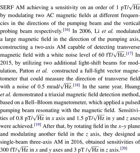
whereγdenotes gyromagnetic ratio of potassium,Rpindicates pumping rate,sindicates the optical-pumping vector along ˆzaxis, andRrelis total relaxation determined by spin exchange collision,spin destruction,and so forth.In the case of a slowly varying magnetic fieldB,by setting dP/dt=0,we can obtain the steady-state solution of the ˆx-componentPxas
(1)通过了解与铁相关的近几年高考试题中的具体生活化内容题材,感受铁及其化合物知识在生产、生活中的重要性。
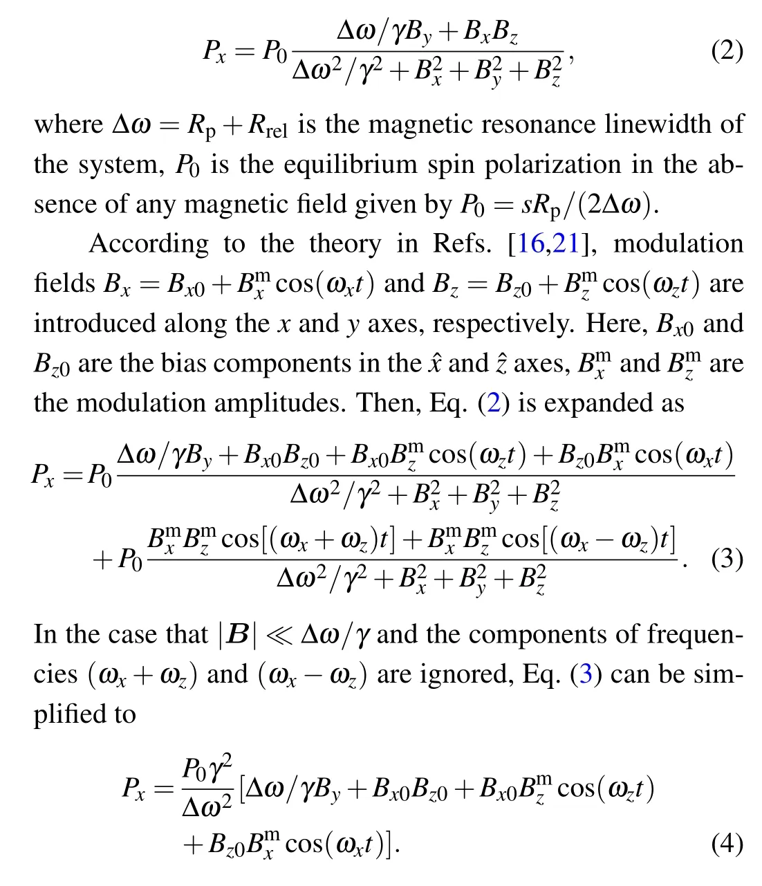
ThusBx0andBz0can be demodulated from the components of frequenciesωzandωxinPx,respectively.If the magnetic field canceling feedback loops are established,Bx0andBz0can be treated as zero andBycan be obtained from DC component.
Equation (3) indicates that the response of demodulated signals toBx0andBz0are both given by a dispersive curve.The sensitivities ofBx0andBz0depend on the slope at the center of the dispersive curve.The amplitude of the dispersive curve is independent of the modulation frequencies according to Eq.(3).In order to improve the response speed of the magnetic field cancelation feedback and to suppress the power line frequency noise and its harmonics, the modulation frequencies should be as high as possible.However, the actual response of the system will deviate from the quasi-steady-state solution as the modulation frequencies increase.The form of the response and its relationship with modulation frequencies should be discussed further.To simplify the problem,we discuss the responses of the two modulations separately and only consider the response at the fundamental frequency.
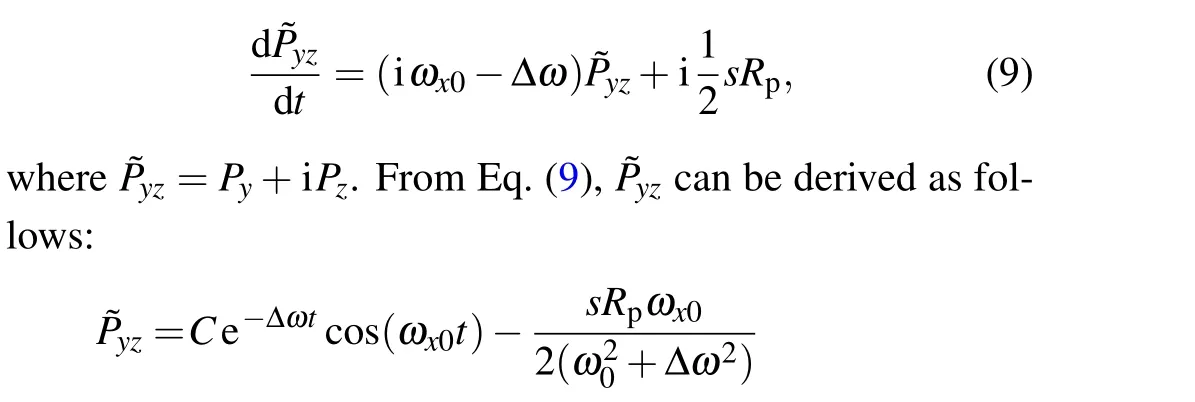
3.2.Response to Bz0 given by frequency-dependence solution
Considering the condition that a bias magnetic field along ˆzaxisBz0=ωz0/γˆzand bias magnetic fields of other axes is zeroed.The transverse components of the spin and transverse magnetic field can be written in the complex form as
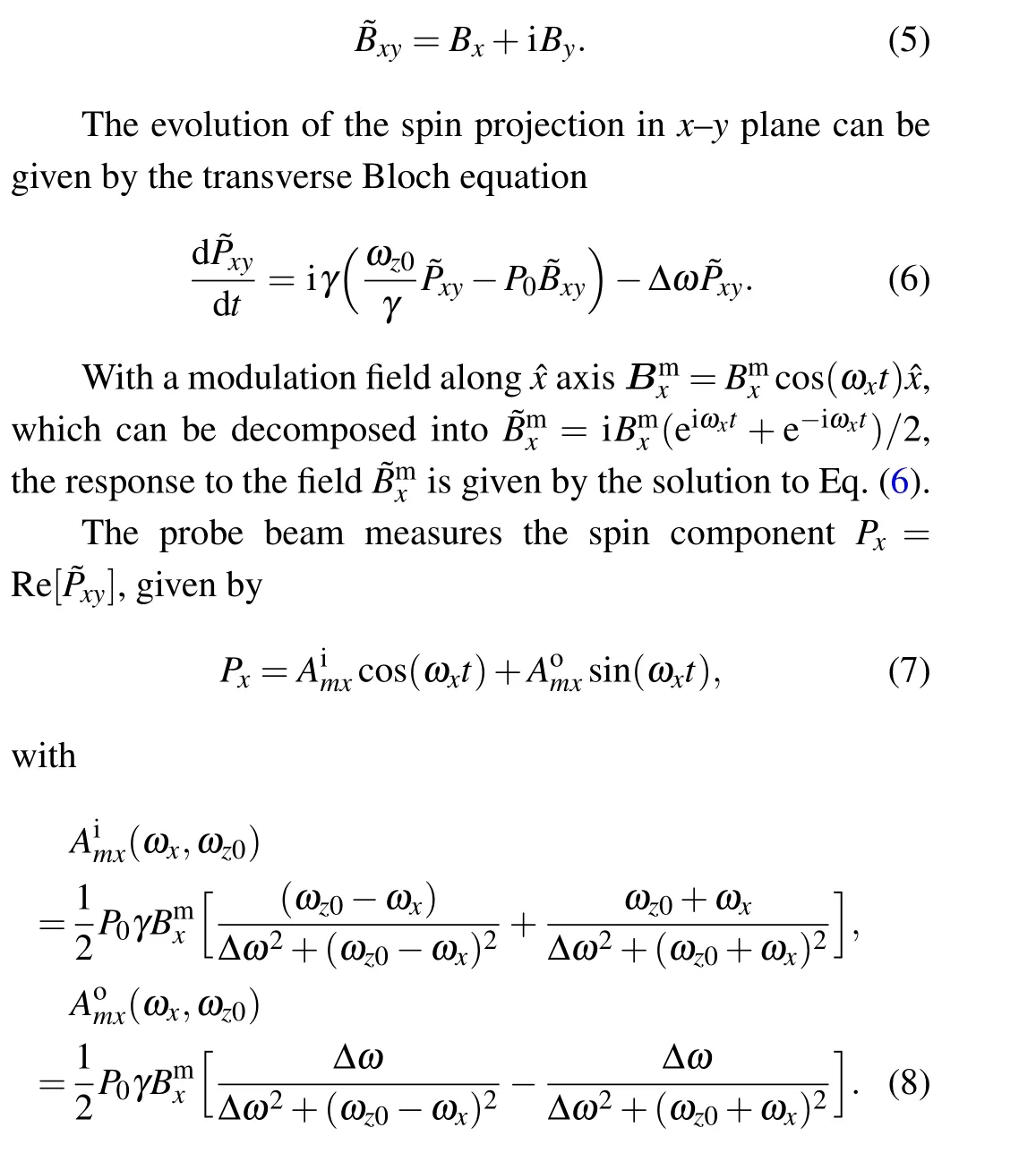
From Eq.(8), the responses of in-phase componentAimxor out-of-phase componentAomxto magnetic fieldsBz0=ωz0/γis given by two overlapping dispersive or Lorentzian curves centered at +ωx/γand-ωx/γ, respectively.The numerical calculation results of Eq.(8)are given in Fig.2.
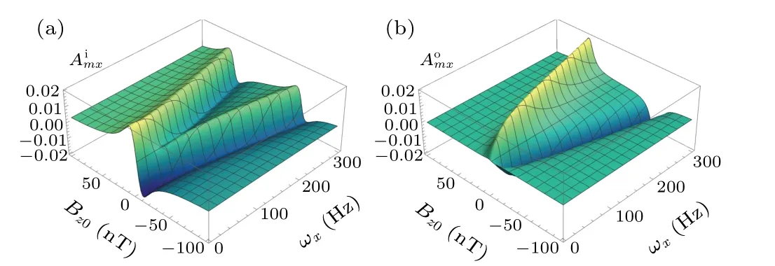
Fig.2.The numerically analyzed result of Eq.(8) with ∆ω =50 Hz in the ranges of Bz0 ∈[-100,100] nT and ωx ∈[1,300] Hz.(a) The in-phase component Aimx demodulated from Px as a function of ωx and Bz0.(b) The out-of-phase component Aomx demodulated from Px as a function of ωx and Bz0.
3.3.The response to Bx0 given by frequency-dependence solution
Considering that a bias magnetic field along ˆxaxisBx0=ωx0/γˆxand bias magnetic field of ˆyand ˆzaxis are zeroed,the spin polarization precesses around the ˆxaxis.We can give the transverse Bloch equation iny–zplane as follows:
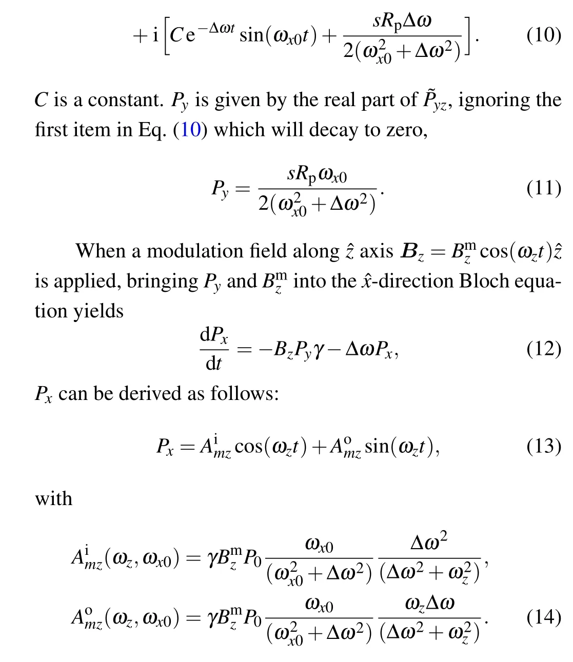
From Eq.(14),the responses of in-phase componentAimzor out-of-phase componentAomztoBx0=ωx0/γare given by a dispersion curve centered at zero,whose amplitude depends on the modulation frequencyωzin a form of Lorentzian or dispersive shape,as shown in Fig.3.

Fig.3.The numerically analyzed result of Eq.(14) with ∆ω =50 Hz in the ranges of Bx0 ∈[-100,100] nT and ωz ∈[1,300] Hz.(a) The in-phase component Aimz demodulated from Px as a function of ωz and Bx0.(b) The out-of-phase component Aomz demodulated from Px as a function of ωz and Bx0.
4.Result and discussion
In order to measure the response of the magnetometer more precisely and offer the condition of the SERF regime,the residual magnetic field in the shielding cylinder was canceled further by the triaxial compensation coils.Modulation fields are applied in ˆxand ˆzaxes in turn according to Eq.(4).The modulation frequency is set to 3 Hz to ensure the validity of the quasi-steady-state solution.The applied compensation fields are adjusted by detecting the components of DC or 3 Hz.The specific process is as follows: First, the modulation field is applied on ˆxaxis,and the bias field on ˆzaxis is adjusted to minimize the 3 Hz component in the output signal.Likewise,the bias field on ˆxaxis is adjusted to minimize the 3 Hz component when the modulation field is applied on ˆzaxis.Then the bias field on ˆyis adjusted to zero of the DC component.In actual operation, the offset of one axis may need to be readjusted after the offset of the other axis is changed.Therefore,we repeat this process until the offsets on all three axes become stabilized.In subsequent experiments,we take this state as the zero magnetic field point.
When the magnetic field offsets of the other two axes are canceled,by setting the corresponding terms in Eq.(2)to zero,the response to the bias field on ˆyaxisBy0can be given by
It can be seen from Eq.(15)that the response toBy0is in the form of a dispersion curve.By scanningBy0, we measured this response as shown in Fig.4.The fitting results of this response indicate that,within the gyromagnetic ratio range of 4.7–7, the magnetic resonance linewidth ∆ωof the system is between 40 Hz and 60 Hz.

Fig.4.The magnetometer response obtained by scanning By0 and the curve of fitting by Eq.(15).
To observe the response forms of theBx0andBz0and their relationships to the modulation frequency,a series of modulation fields at different frequencies are applied in the ˆxand ˆzaxes respectively,andBx0orBz0are swept accordingly.With 5 Hz,60 Hz,and 600 Hz modulations on ˆxaxis,the scanning results ofBz0and the fitting results of Eq.(8) are shown in Figs.5(a),5(b),and 5(c).With 5 Hz,40 Hz,and 600 Hz modulations on ˆzaxis, the scanning results ofBx0and the fitting results of Eq.(14)are shown in Figs.5(d),5(e),and 5(f).
We could find that the in-phase signals reach the maximum, and the out-of-phase signals will approach zero when the modulation frequencies are much lower relative to ∆ω,no matter whether it is for modulations along the ˆxaxis or the ˆzaxis.This implies that the responses converge to the quasisteady-state solution.Under the condition that the modulation frequencies are close to the linewidth ∆ω, the in-phase signal responding to the modulation in ˆxaxis is insensitive toBz0near zero meanwhile the slope of the out-of-phase signal is maximized.The in-phase and out-of-phase signals responding to the modulation in ˆzaxis perform equal amplitude.In our experiments, the frequency with equal in-phase and outof-phase signal amplitudes occurs at 40 Hz, which differs by about 15 Hz from the magnetic resonance linewidth measured byBy0scanning.One of the reasons may be that we neglected the difference of the polarization relaxation times in the ˆzaxis direction and inx–yplanes in our calculations.In the case that the modulation frequency is much larger than the linewidth∆ω, the slope of the out-of-phase signal near the zero magnetic field is larger than the in-phase signal.However,they are both attenuated a lot in two modulations.
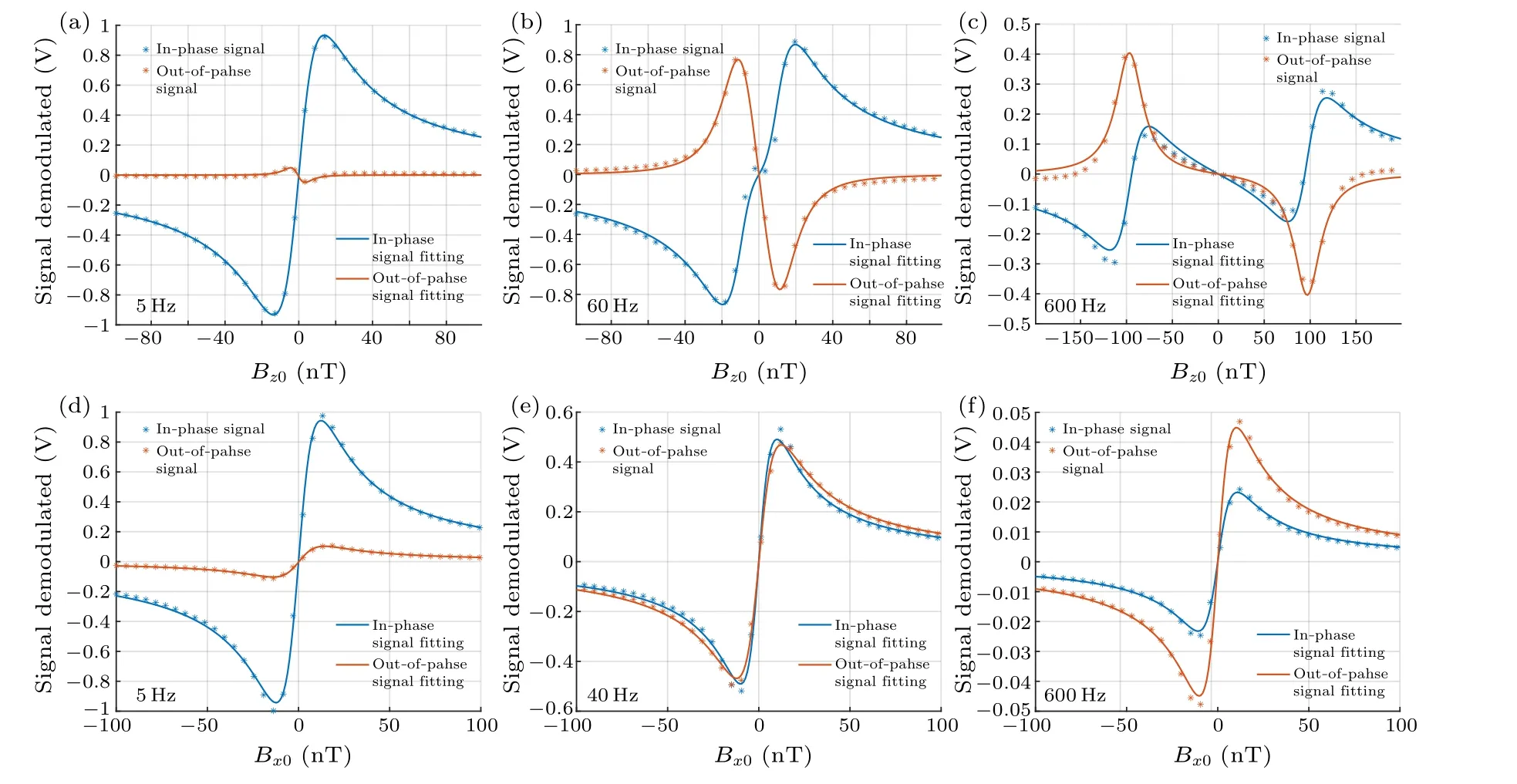
Fig.5.The system responses to Bz0 and Bx0 under different modulation frequencies.(a)The response to Bz0 with modulation field of 5 Hz in ˆx axis.(b)The response to Bz0 with modulation field of 60 Hz in ˆx axis.(c)The response to Bz0 with modulation field of 600 Hz in ˆx axis.(d)The response to Bx0 with modulation field of 5 Hz in ˆz axis.(e)The response to Bx0 with modulation field of 40 Hz in ˆz axis.(f)The response to Bx0 with modulation field of 600 Hz in ˆz axis.
In addition,we further investigate the frequency response of the system to the triaxial magnetic field components.For unshielded applications,the frequency response of the magnetometer is also important because it is directly related to the bandwidth that the magnetic field feedback compensation system can achieve.
In the solutions given in Subsections 3.2 and 3.3, we only considered the fundamental frequency components of the modulation frequencies.However, for the actual signal,there are not only the harmonics of the modulation frequencies but also the sum and difference frequency components of the two modulation frequencies,which are also been indicated by Eq.(3).
To compromise between the amplitude of the signal and the bandwidth that can be achieved after demodulation, the modulation frequency in ˆxaxis is set to 150 Hz and that in ˆzaxis is set to 250 Hz,which also ensures that there will be no spurious signals caused by modulation within the frequency band of 100 Hz.The effective values of the modulation signals are all 20 nT.The time constants of the two lock-in amplifiers are both set to 3 ms and the filter slopes are set to 6 dB.The same parameters are applied for the low-pass filter which extracts the ˆyaxis signal.Another lock-in-amplifier is used to apply AC magnetic fields with an effective value of 1 nT on three axes sequentially.The fields are offered by the selfcontained coils by the shielding cylinder which is composed of a solenoid and two sets of saddle coils, and are not shown in Fig.1.The frequency of the fields is swept in the range of 1–100 Hz to test the frequency response of demodulated signal to the triaxial magnetic field components, and the results are shown in Fig.6.
The in-phase and out-of-phase components in the frequency response of the ˆyaxis magnetic field are in the forms of Lorentzian and dispersion curves, respectively, which are given by[21]
whereF(ω) is the fitted function,Kis the amplitude, ∆ωis the linewidth,ω0is the peak position, andCis the baseline offset.
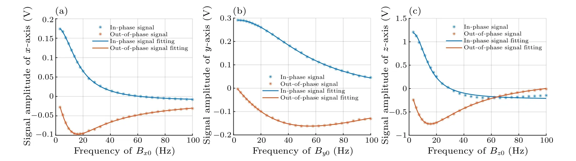
Fig.6.The open-loop frequency response of demodulated signal to the triaxial magnetic field components.(a)The frequency response to ˆx axis component.(b)The frequency response to ˆy axis component.(c)The frequency response to ˆz axis component.
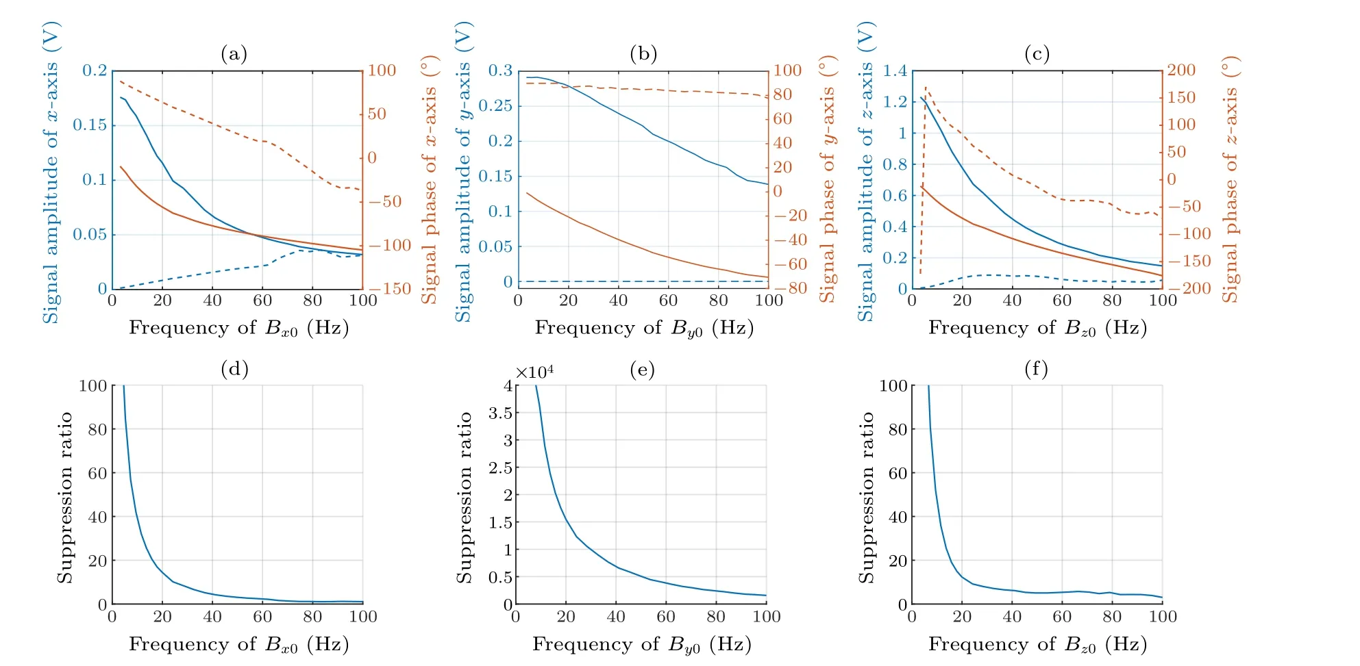
Fig.7.The closed-loop frequency response of the amplitude and phase of the signal to the triaxial magnetic field components compared with the open-loop response.The open-loop responses are marked with solid lines, and the closed-loop responses are marked with dashed lines.Blue represents the magnitude response and red represents the phase.(a)The frequency response to ˆx axis component.(b)The frequency response to ˆy axis component.(c)The frequency response to ˆz axis component.(d)The inhibition ratio to ˆx axis component.(e)The inhibition ratio to ˆy axis component.(f)The inhibition ratio to ˆz axis component.
Interestingly,for the demodulated signals of ˆxand ˆzaxes,the in-phase and out-of-phase components in their frequency responses can also be well fitted by Lorentzian and dispersive curves.It should be noted that in this test,the signal of ˆxaxis which is demodulated from the modulation in ˆzaxis is given by the out-of-phase component,because at the set modulation frequency the amplitude of the out-of-phase signal is much larger than that of the in-phase signal.The signal of ˆzaxis which is demodulated from the modulation in ˆxaxis is given by the in-phase component because of its larger amplitude.Of course,the signal amplitude can be maximized by optimizing the demodulation phase.Herein, we tend to show this result which is in good agreement with the Lorentzian and dispersion curves in the experiments.The signal amplitude improvement brought from the phase optimizing will not be too much.This suggests that a uniform control algorithm can be employed for providing feedback control to magnetic fields in all three directions,requiring parameter adjustments exclusively.
Based on the frequency response results given above,we design the three-axis magnetic field feedback compensation.The PID control algorithm is implemented by the microcontroller,and the three-way output signals of the system are read by the three analog-to-digital converters(ADCs)directly controlled by the microcontroller, due to the real-time requirements of the feedback system.The test magnetic fields are still provided by the shielding cylinder’s own coils and are still swept in the range of 1–100 Hz.After the closed-loop compensation is established,the frequency response of the system is measured again, as shown in Fig.7.For comparison, the results without feedback compensation are also shown again in Fig.7 in the form of bode plot(in comparison with the inphase and out-of-phase signals in Fig.6, here the Bode plot system is used to compare the system responses).Additionally, the proportional relationship between the two response curves is utilized to showcase the attenuation ratio.Utilizing the mentioned modulation frequencies and operating within the vicinity of the DC frequency range, a remarkably pronounced suppression effect on the magnetic field becomes evident.Notably,the suppression ratios for the ambient magnetic fields exceed 10 times within the frequency band below 20 Hz along all three axes.The ratios are not less than 3 and 5 times at 50 Hz in ˆxand ˆzaxes.The capability of the suppression to power line noise shows the potential of the system to operate in a completely unshielded environment.
5.Conclusions
In this work,a model describing the response of the threeaxis SERF magnetometer under high frequency modulations is presented and verified experimentally,which can serve as a reference for modulation frequency selection.We observe a magnetic resonance linewidth of approximately ∆ω ≈55 Hz.Across the specified modulation frequency,the suppression ratios for all three axes relative to the ambient magnetic field exceed 10 within the frequency range below 20 Hz.At 50 Hz,the suppression ratios along thexandzaxes are at least 3 and 5 times, respectively.The magnetic field canceling experimental result shows an ability to suppress power frequency noise of the system,which reflects its potential to operate in a geomagnetic field environment without heavy aluminum shielding.
Acknowledgment
Project supported by the National Natural Science Foundation of China(Grant No.42074216).
猜你喜欢
中学生数理化·自主招生(2022年2期)2022-05-30
中学生数理化(高中版.高考理化)(2022年2期)2022-04-26
中学生数理化·中考版(2021年12期)2021-12-31
中学生数理化·中考版(2021年11期)2021-12-06
中等数学(2020年4期)2020-08-24
中学数学杂志(2019年1期)2019-04-03
中学化学(2017年6期)2017-10-16
校园英语·下旬(2016年7期)2016-07-28

- Chinese Physics B的其它文章
- Unconventional photon blockade in the two-photon Jaynes–Cummings model with two-frequency cavity drivings and atom driving
- Effective dynamics for a spin-1/2 particle constrained to a curved layer with inhomogeneous thickness
- Genuine entanglement under squeezed generalized amplitude damping channels with memory
- Quantum algorithm for minimum dominating set problem with circuit design
- Protected simultaneous quantum remote state preparation scheme by weak and reversal measurements in noisy environments
- Gray code based gradient-free optimization algorithm for parameterized quantum circuit