MetaPINNs: Predicting soliton and rogue wave of nonlinear PDEs via the improved physics-informed neural networks based on meta-learned optimization

Yanan Guo(郭亚楠), Xiaoqun Cao(曹小群), Junqiang Song(宋君强), and Hongze Leng(冷洪泽)

1College of Meteorology and Oceanography,National University of Defense Technology,Changsha 410073,China

2College of Computer,National University of Defense Technology,Changsha 410073,China

3Naval Aviation University,Huludao 125001,China

Keywords: physics-informed neural networks, gradient-enhanced loss function, meta-learned optimization,nonlinear science

1.Introduction

In recent years, with the rapid development of artificial intelligence technology, especially deep learning, many fields have undergone significant transformations.Currently,deep learning technology has achieved remarkable milestones across various domains,including object detection,autonomous vehicles, and time series analysis.[1–3]Moreover,deep learning techniques are progressively shifting from being solely data-driven to being driven by the fusion of data and knowledge.It is worth paying attention to the rapid development of this research direction,and the related algorithms are beginning to penetrate into various fields.In the realm of scientific research,deep learning methods are becoming increasingly indispensable as research tools, profoundly advancing scientific discoveries,theoretical derivations,and other related research.They are exerting a rapid and profound influence on the development of disciplines such as physics, mathematics,materials science,and geosciences.[4–7]

So far,scientific research driven by deep learning has resulted in a multitude of noteworthy accomplishments.For example, one notable application of deep learning methods has been in the field of weather and climate prediction, where it has substantially improved the accuracy of forecasts, particularly for highly impactful weather events like super typhoons and extreme precipitation.[8,9]Another exciting area of advancement is the utilization of deep neural networks for solving various types of partial differential equations (PDEs)and modeling complex natural physical phenomena.[10–13]In this context, Raissiet al.introduced the concept of physicsinformed neural networks (PINNs), which represents an improvement over traditional neural network-based methods for solving forward and inverse problems of partial differential equations.Numerous studies have shown that PINNs can effectively integrate the intrinsic constraint information in the physical equations.[14]Physics-informed neural networks serve as a comprehensive framework that combines datadriven and knowledge-driven approaches for modeling physical phenomena.PINNs differ from traditional neural networks in their unique ability to seamlessly incorporate the physical constraints of PDEs.This innovative approach reduces the need for extensive training data and enhances the interpretability of the model.PINNs are characterized by a flexible loss function that allows for the integration of PDE constraints, as well as boundary and initial condition constraints, in addition to observational data constraints.In recent years, a multitude of researchers have dedicated significant efforts to the study and enhancement of PINNs, introducing various innovative variants and applying them across diverse domains, including mechanics, geology, oceanography, and meteorology.[15–18]For example, Chenet al.proposed a variable coefficient physics-informed neural network(VC-PINN),[19]which specializes in dealing with the forward and inverse problems of variable coefficient partial differential equations.Caoet al.adopted an adaptive learning method to update the weight coefficients of the loss function for gradientenhanced PINNs and dynamically adjusted the weight proportion of each constraint term,[20]and numerically simulated localized waves and complex fluid dynamics phenomena,which achieved better prediction results than the traditional PINNs,and the improved method also performed well for the inverse problem under noise interference.

Solitary waves and rogue waves represent the distinctive phenomenon frequently observed in various natural environments,[21–24]including the atmosphere and oceans.This research area is a cross-discipline of atmospheric science,ocean science,applied mathematics,and engineering technology and is considered an essential frontier research with farreaching theoretical significance and application prospects.[25]Consequently, solitary waves and rogue waves have emerged as a pivotal focus within the realm of geophysical fluid dynamics, spurring extensive theoretical exploration and highprecision simulation endeavors.However, traditional numerical computation methods encounter challenges such as low computational efficiency, substantial computational resource requirements, and error accumulation.Therefore, there is a growing imperative to explore novel numerical simulation techniques.For example, Chenet al.successfully solved the soliton solution of the nonlocal Hirota equation using a multilayer physics-informed neural network algorithm and investigated the parameter discovery problem of the nonlocal Hirota equation from the perspective of the soliton solution.[26]In addition, Chenet al.designed a two-stage PINN method based on conserved quantities that can impose physical constraints from a global perspective,[27]and applied it to multiple types of solitary wave simulations.Numerical results show that the two-stage PINN method has higher prediction accuracy and generalization ability compared with the original PINN method.Liet al.combined mixed-training and a priori information to propose mixed-training physicsinformed neural networks (PINNs) with enhanced approximation capabilities,[28]and used the model to simulate rogue waves for the nonlinear Schrödinger (NLS) equation, and the numerical results show that the model can significantly improve the prediction accuracy compared with the original PINNs.Even when the spatio-temporal domain of the solution is enlarged or the solution has local sharp regions,the improved model still achieves accurate prediction results.Furthermore, Liet al.simulated higher-order rogue waves of the cmKdV equation using mixed-training physicsinformed neural networks (MTPINNs) and mixed-training physics-informed neural networks with a priori information(PMTPINNs),[29]which showed significantly better prediction accuracy compared to the original PINNs.In addition, these models have reliable robustness for the inverse problem under noisy data.In this study, we introduce a new structure and loss function specifically designed for modeling solitary and rogue wave phenomena using physics-informed neural networks.We conduct a comprehensive investigation into the simulation of solitary waves and rogue waves employing these enhanced PINNs and validate our approach through a series of numerical experiments.

2.Methodology

2.1.Physics-informed neural networks

Physics-informed neural networks are a class of neural networks used for addressing supervised learning tasks while simultaneously adhering to the physical laws described by partial differential equations.As a machine learning method applied in the scientific computing, PINNs are employed to tackle a wide range of issues related to partial differential equations,encompassing approximate solutions of these equations, parameter inversion, model discovery, control, optimization, and more.After PINNs were proposed, a large amount of follow-up research work was triggered, and they gradually became a research hotspot in the emerging crosscutting field of scientific machine learning.From the perspective of mathematical function approximation theory,neural network can be regarded as a general nonlinear function approximator, and the modeling process of partial differential equations is also to find nonlinear functions that satisfy the constraints, which are quite consistent with each other.The neural network trained in this way not only approximates the observed data,but also automatically satisfies the physical properties of symmetry,invariance,and conservation followed by the partial differential equations.The following section describes the design method of PINNs using a partial differential equation in generalized form as an example.Let the functionu=u(x,t)satisfies a partial differential equation of the following form:

whereN(u,λ)is a generalized function with parameterλthat performs differential operation onu,xis a spatial variable,tis a temporal variable,Ωis a subset of the Euclidean space,andTis the termination moment.The traditional physical model is that given the initial conditions, boundary conditions and physical parameterλofu(x,t), the value of theu(x,t)at any point in time and space can be predicted by solving the partial differential equation, and when an analytical solution is not available, it can be solved by using numerical methods, such as finite difference method and finite element method,etc.The PINNs consider the establishment of a neural networku(x,t)to approximate the solution of the partial differential equation.f(t,x)=ut+N(u,λ) is the residual of the partial differential equation, and the loss function of the PINN is defined as Loss=Lo+LIC+LBC+LPDE,where

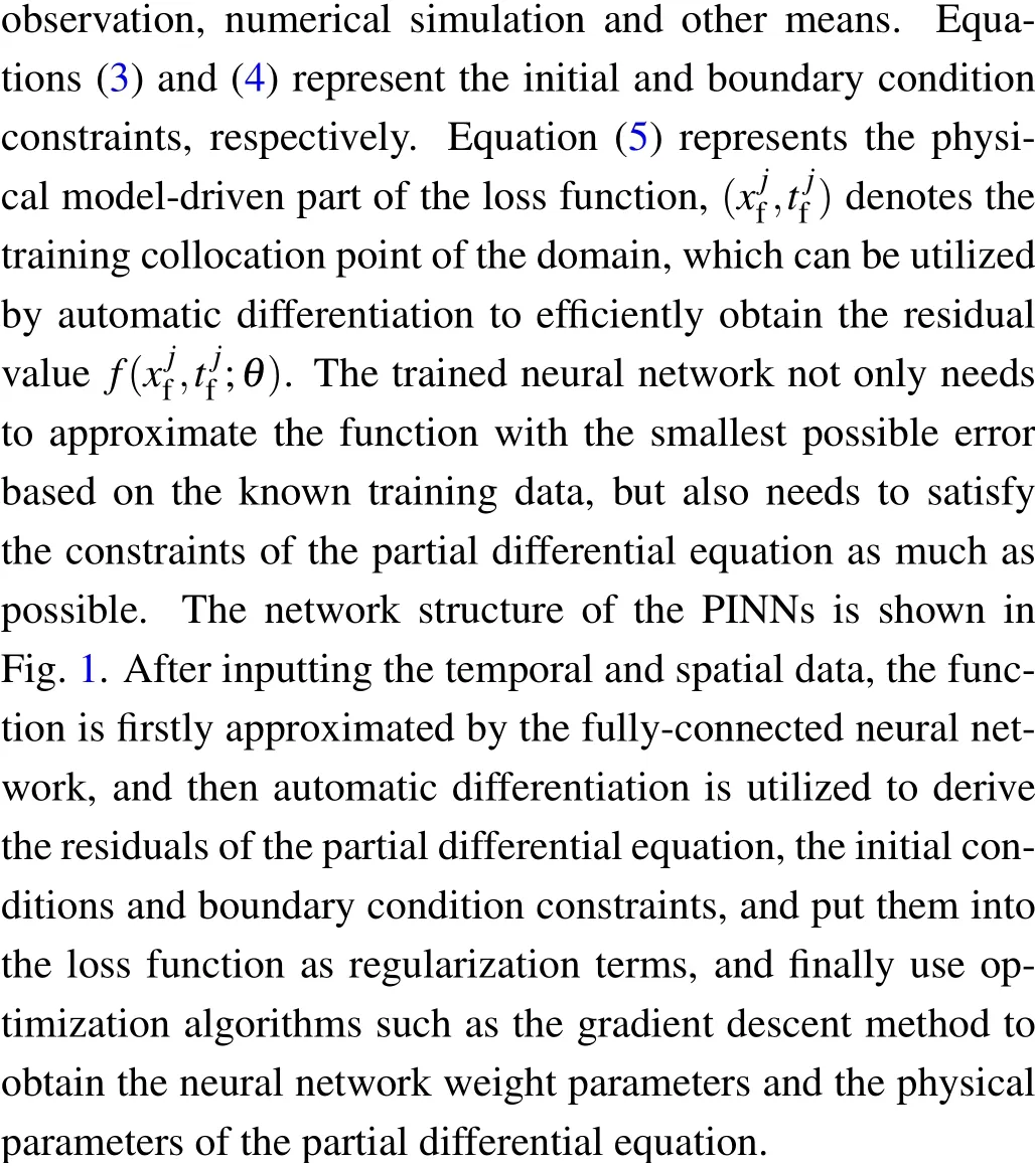
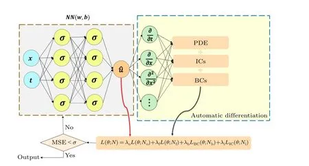
Fig.1.Schematic of physics-informed neural networks for solving partial differential equation.

2.2.Meta learning

While traditional deep learning methods use fixed learning algorithms to solve problems from scratch,meta-learning aims to improve the learning algorithm itself, which avoids many of the challenges inherent in deep learning, such as data and computational bottlenecks, and generalization problems.Meta-learning is divided into three main categories,namely metrics-based approaches, model-based approaches,and optimization-based approaches.Metric-based approaches learn a metric or distance function within a task,while modelbased approaches design an architecture or training process for fast generalization across tasks.Optimization-based methods achieve fast tuning by adjusting the optimization function using only a small number of samples.The framework of meta-learning is widely used in small-sample learning,and its core idea is to learn generalized prior knowledge on similar learning tasks so that only a few samples are needed, and the prior knowledge is used to quickly fine-tune on a new task to achieve the desired result.Therefore,the key of meta-learning is to discover the universal laws between different problems and utilize the universal laws to solve new tasks and problems.The universal laws need to achieve a balanced representation of the generalities and characteristics of the tasks.The search for universal laws mainly relies on the following points.

(i) Discovering and summarizing the links between already solved problems and new problems, and extracting the universal laws of already solved problems for use in solving new problems.

(ii)Decomposing and simplifying the new problem,finding universal laws in the already solved problem that are closely linked to the various subtasks of the new problem,and analyzing the scope of application of these laws.

(iii)Learning logical reasoning in new tasks,using logical reasoning to make representations of new problems, finding laws in these representations, and finding solutions to complex new tasks through logical reasoning between the parts of the new problem.

Meta-learning is essentially a bilevel optimization problem,where one optimization problem is nested within another optimization problem.The external optimization problem and the internal optimization problem are often referred to as the upper level optimization problem and the lower level optimization problem, respectively.The two-layer optimization problem involves two participants: the upper layer participant is the meta-learner and the lower layer participant is the baselearner.The optimal decision of the meta-learner depends on the response of the base-learner,which itself optimizes its own internal decisions.These two levels have their own different objective functions, constraints and decision variables.The objects and functions of the base-learner and meta-learner are shown in Fig.2.Base-learner is the model in the base layer.The data set on a single task is considered while training the base-learner each time.Meta-learner is the model in the metalayer that summarizes the training experience on all tasks.After training the base-learner each time, the meta-learner synthesizes the new experience and updates the parameters in the meta-learner.The main purpose of meta-learning is to find the meta-learnerF, under the guidance ofF, the base-learnerqcan get the optimal stateq*adapted to the current new task after a few steps of fine-tuning under the support setDtr.And the optimization ofFrequires the cumulative sum of the losses of all current tasks,i.e.,∇∑Nn=1l(qn,Dten).The meta-learning works as shown in Fig.3.

Fig.2.Schematic diagram of the base-learner and the meta-learner.

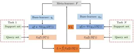
Fig.3.The schematic of meta learning’s working mechanism.

2.3.The improved physics-informed neural networks

In the original PINNs,only the PDE residualsfare constrained to be zero.However, upon further analysis, it becomes evident that iff(x) is zero for anyx, then its derivative,∇f(x),is also zero.Therefore,we make the assumption that the exact solution of the PDE possesses sufficient smoothness to warrant the existence of the gradient of PDE residuals, ∇f(x).Consequently, we introduce gradient-enhanced PINNs, where not only are the PDE residuals zero, but also their derivatives, as described mathematically by the following equation:[30]

Based on the aforementioned definition, it is inherent to derive the loss function for gradient-enhanced PINNs

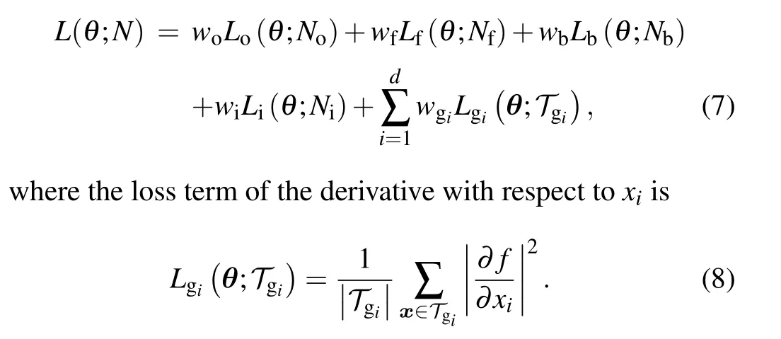
Here,Tgirepresents the set of residual points for the derivative∂f/∂xi.It is important to emphasize thatTgi(fori=1,2,...,d)may vary between different equations.To enhance the generalization capabilities of PINNs,this study integrates meta-learning into their training process.

While the original optimizer uses manually designed optimization rules,such as the Adam optimizer for updating the weight vectorθof a physics-informed neural network with loss functionL(θ),meta-learning can improve upon these previously manually designed optimization rules.Specifically,the original Adam update rule is as follows:

wheremtandvtare the first and second moments at time stept, respectively, withεbeing a small regularization constant used for numerical stability,β1,β2∈[0,1)being the exponential decay rates for the moment estimates, andηbeing the learning rate.The meta-learned optimizer’s parameters undergo updates through the following process:

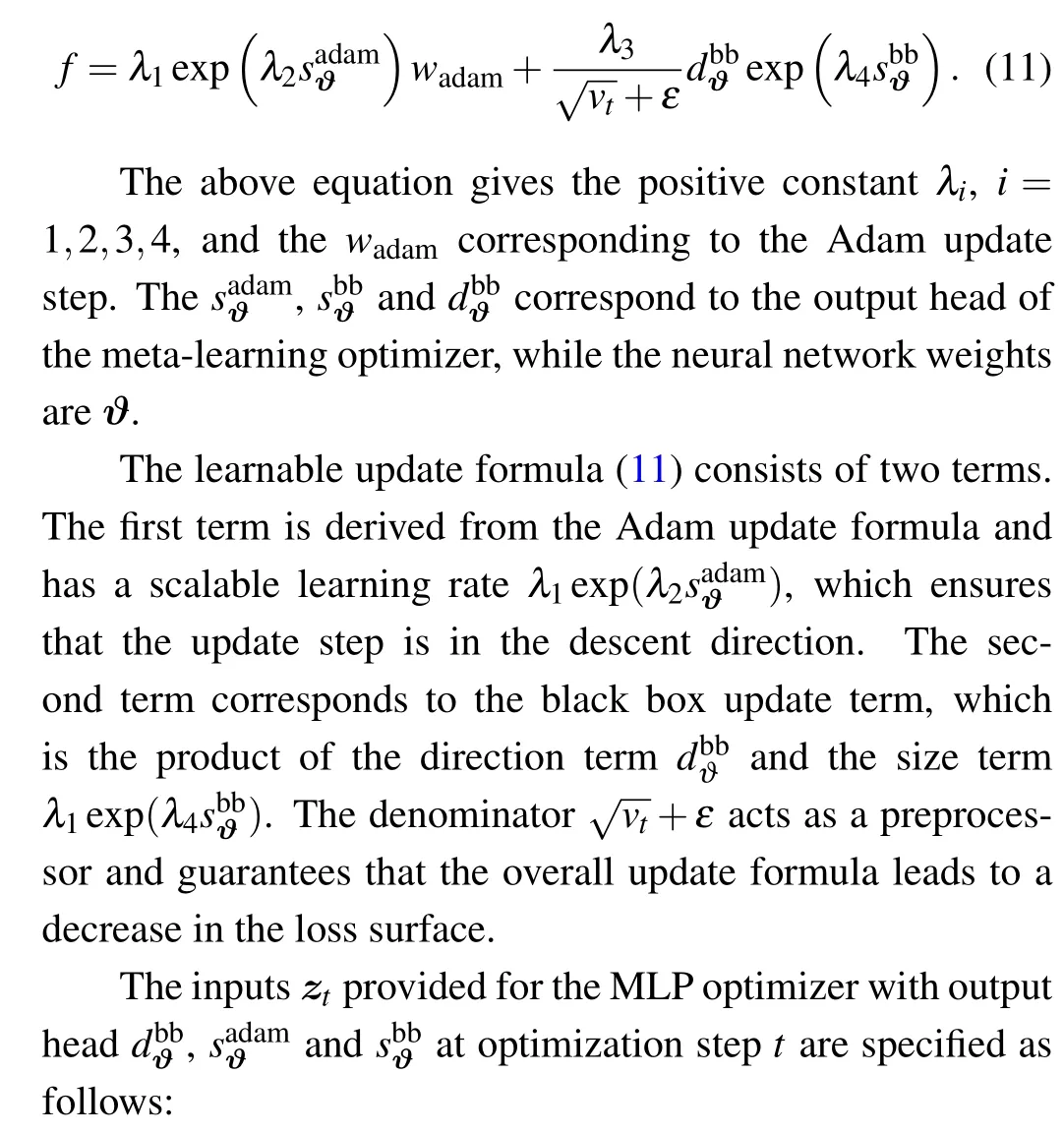
wherefis the parameter update function of the learnable optimizer,ztis the input feature, andϑis the trainable metaparameter.For the component form,each parameterθiof the updated parameter vectorθis computed in the same way.The optimizer architecture used in this study utilizes a multilayer perceptron (MLP), which is simple, but better illustrates the potentiality of the approach in this paper.Specifically,the update formula for each parameterθiis as follows:

(i)The neural network weightsθt.

(ii)The gradients of loss function ∇θL(θt).

(iii) The second momentum accumulatorsvtwith decay ratesβ2∈{0.5,0.9,0.99,0.999}and inverse of the square root of these second momentum accumulators.

(iv)The time stept.

The present study improved physics-informed neural networks by utilizing the aforementioned input parameters.All input features, except for the time step, were normalized such that one of their second-order moment was equal to 1.The time step was transformed into a total of eleven features by computing tanh(t/x), wherex ∈{1,3,10,30,100,300,1000,3000,10k,30k,100k}.Subsequently, all features were concatenated and inputted into the MLP to produce the aforementioned three output heads.

3.Numerical experiments and results

In this section,we conduct experiments to investigate the solitary wave and rogue wave phenomena utilizing gradientenhanced PINNs with meta-learned optimization.Specifically,we seek to approximate the solitary wave solutions of the Kaup–Kuperschmidt (KK) equation and rogue waves of the nonlinear Schrödinger equation.At the end of model training,we quantitatively evaluate the performance of the enhanced PINN model for solitary wave and rogue wave simulation.This assessment encompasses an in-depth analysis of its convergence rate and the accuracy of the prediction results.The accuracy of the approximate solutions generated by the enhanced PINN model is quantified using the L2 norm relative error,defined as follows:

whereNrepresents the number of grid points, ˆu(xi,ti) indicates the approximate solution generated by the neural network model,andu(xi,ti)represents the exact solution.

3.1.Numerical simulation of solitary wave of the Kaup–Kuperschmidt equation

Next, we conduct experimental research on the Kaup–Kuperschmidt equation,[31,32]which is mathematically defined as follows:

The KK equation is commonly used to describe the evolution and nonlinear effects of water waves.It has a wide range of applications, including oceanography, fluid dynamics, and nonlinear optics,making it an important tool for studying various nonlinear wave phenomena.Meanwhile,researchers have found that the KK equation can support multiple solutions,including solitary waves and other nonlinear wave solutions,which play a crucial role in the propagation and evolution of water waves.However,the study and analysis of the KK equation are typically very complex because it is a highly nonlinear partial differential equation.

For Eq.(13),we meticulously defined our numerical simulation parameters, limiting our spatial exploration to the interval [-20,20] and our temporal investigation to the period[-5,5].These parameter choices were guided by careful consideration of the following set of initial condition and boundary condition:

In accordance with the previously stated conditions, the solitary wave solution of the KK equation is expressed as follows:

whereθ1=k1x-k51tandu(x,t)describes the amplitude of the wave at positionxand timet.

To effectively approximate the precise solution of the KK equation,we employed a neural network architecture consisting of five hidden layers,each comprising 64 neurons.In terms of the initial and boundary conditions,we generated a training dataset through random sampling, incorporating 400 samples.We selected random spatiotemporal locations to calculate residuals, facilitating the formulation of physical constraints.A total of 15000 data points were sampled during the experiment.Furthermore, a limited set of observations, consisting of 400 data points,was employed.Utilizing these data samples, we devised a composite loss function.We utilized a learnable optimizer to optimize the loss function, with the optimizer’s constant set asλj=10-4.Following the training process, the neural network model was employed to approximate the solitary wave solution of the Kaup–Kuperschmidt equation.In Fig.4,both the exact solution and the predictions generated by the trained model are presented.From Fig.4,it is evident that the enhanced PINNs can accurately predict the precise solution of the KK equation with high precision.Subsequently,for a detailed analysis of the experimental outcomes, we selectively examine the prediction results at different moments, comparing them with the exact solution to assess the accuracy of the improved PINNs.Figure 5 provides a visual representation of the comparison between the exact solution and the approximated solution at different times.The prediction values generated by the enhanced PINNs closely match the exact solutions, signifying a noteworthy degree of accuracy.Furthermore, following multiple experiments, we quantify the disparities between the approximate solution and the exact solution.The L2 norm relative error between the predictions generated by the enhanced PINNs and the exact solution is approximately 8.20×10-4.With the same training data and parameter configurations, the L2 norm relative error between the predictions made by the original PINNs and the true solution is approximately 5.22×10-3.Figure 6 displays the error statistics for both the improved PINNs and the original PINNs.Furthermore, we conduct an analysis of the model’s training time before and after the enhancements.The results indicate that the enhanced PINNs complete the training process in approximately 47.6%of the time required by the original PINNs.To more thoroughly analyze the effects of the number of neural network layers,the number of neurons and the number of collocation points on the prediction solution error, we chose different numbers of the hidden layers,different numbers of neurons and different numbers of collocation points to conduct numerical experiments and compared the prediction solution errors of the original PINNs and the improved PINNs.The experimental results are shown in Table 1.Analyzing the experimental results,it can be found that as the number of neural network layers increases,the number of neurons increases and the number of collocation points increases,the prediction solution error decreases.In addition,it is evident that the improved PINNs exhibit superior training efficiency and yield more accurate prediction outcomes compared to the original PINNs when simulating a single solitary wave of the KK equation.

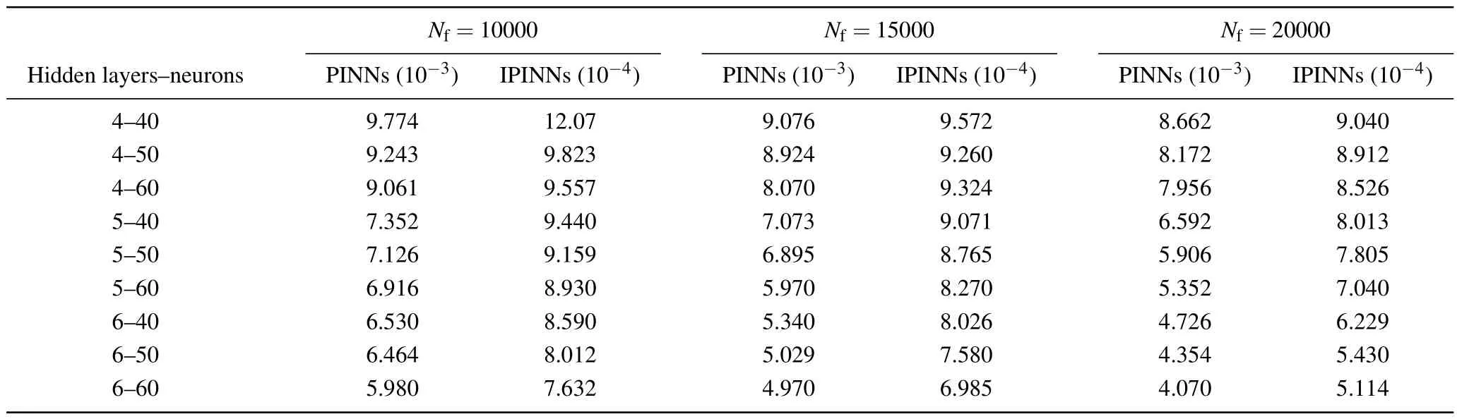
Table 1.For the KK equation,the errors of the predicted solutions are compared at different numbers of the neural network layers,different numbers of neurons,and different numbers of collocation points.

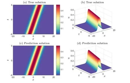
Fig.4.Exact soliton solutions and predicted solutions of the KK equation: (a) two-dimensional visualization of the true solution, (b) threedimensional visualization of the true solution, (c) two-dimensional visualization of the predicted solution of the improved PINNs, (d) threedimensional visualization of the predicted solution of the improved PINNs.

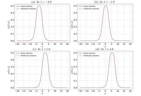
Fig.5.Comparison of the exact solitary wave solution to the predicted solitary wave solution of the KK equation at four different time instances:(a)t=-4.0,(b)t=-1.0,(c)t=1.0,and(d)t=4.0.

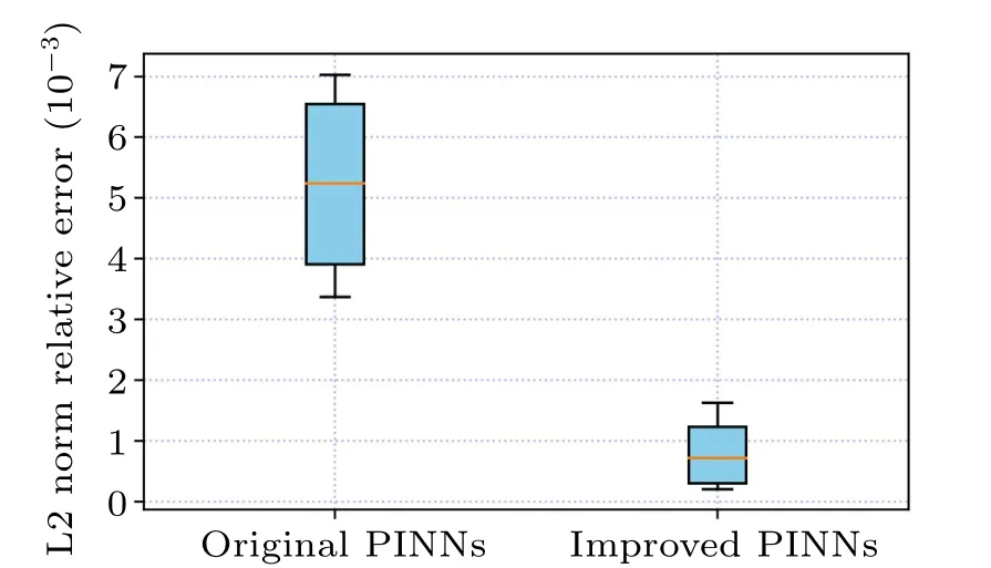
Fig.6.Visual analysis of errors in the prediction results of the solitary wave solution of the KK equation: comparison of the errors of the improved PINNs and the original PINNs.

3.2.Numerical simulation of first-order rogue wave of the nonlinear Schrödinger equation

In order to illustrate the applicability of the improved PINN to rogue wave prediction, we conduct experimental research on the nonlinear Schrödinger equation,[33–35]which is mathematically defined as follows:

The following solution is obtained by the Hirota transfor-mation:

where

In the above equations,Ω(0)nandφnare free complex parameters andkis a real parameter.In this subsection, the value ofkis zero.For the Eq.(18), the study domain for the numerical simulations is set to the spatial range[-5,5]and the time range[-5,5].When choosing these parameters,we carefully consider the following set of initial and boundary conditions:

In the experiment,simulations are performed for the firstorder rogue wave of the nonlinear Schrödinger equation.First,we construct a deep neural network with six hidden layers,each containing 64 neurons.During training,the loss function is optimized using a learnable optimizer with a constant set toλj=10-4.All weights and biases in the model are initialized using the Xavier method.For consistency and ease of performance comparison of subsequent methods, we still use the initial conditions as special Dirichlet boundary conditions on the spatio-temporal domain.It is worth noting that the number of observations is only 400, whereas 10000 collocation points were selected for the construction of the equation constraints and 400 sample points were selected for the construction of the initial condition constraints and boundary condition constraints.Figure 7 compares the difference between the prediction results of the improved PINNs and the true solution.The relatively good prediction results convince us that the improved PINNs can effectively predict the first-order rogue wave of the nonlinear Schrödinger equation.Figure 8 shows the comparison of the prediction results between the exact solutions and the improved PINNs atdifferent moments,and we can find that the two solutions are in high consistency.Similarly,we calculate the L2 norm relative error of the prediction results of the improved PINNs with respect to the true solution,which has a value of 8.33×10-4,while the L2 norm relative error of the original PINNs with the same experimental setup is 6.41×10-3,and the comparison results are given in Fig.9.As for the computational efficiency,the time required for the improved PINNs to complete the training is only 51.6%of the training time of the original PINNs.In this study, we also quantitatively analyze the effects of the number of neural network layers, the number of neurons, and the number of collocation points on the prediction solution of the first-order rogue waves of the nonlinear Schrödinger equation,and select different numbers of hidden layers, different numbers of neurons, and different numbers of collocation points for numerical experiments,and compare the prediction solution errors of the original PINNs and the improved PINNs.The specific experimental results are shown in Table 2.Analyzing the experimental results,it can be found that as the number of neural network layers increases, the number of neurons increases, and the number of collocation points increases,the prediction solution error is also reduced.The experiments can show that the improved PINNs outperform the original PINNs in terms of both computational efficiency and prediction accuracy.

Table 2.For the first-order rogue wave of the nonlinear Schrödinger equation,the errors of the predicted solutions are compared at different numbers of the neural network layers,different numbers of neurons,and different numbers of collocation points.

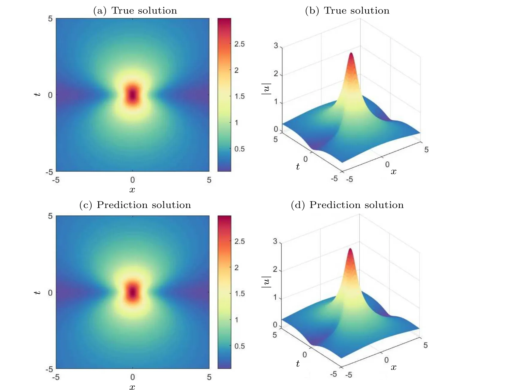
Fig.7.Exact first-order rogue wave solutions and predicted solutions of the nonlinear Schrödinger equation: (a)two-dimensional visualization of the true solution, (b) three-dimensional visualization of the true solution, (c) two-dimensional visualization of the predicted solution of the improved PINNs,(d)three-dimensional visualization of the predicted solution of the improved PINNs.

Fig.8.Comparison of the exact first-order rogue wave solution to the predicted first-order rogue wave solution of the nonlinear Schrödinger equation at four different time instances: (a)t=-3.0,(b)t=-1.0,(c)t=1.0,and(d)t=3.0.

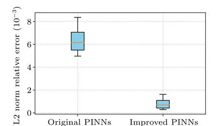
Fig.9.Visual analysis of errors in the prediction results of the first-orderrogue wave solution of the nonlinear Schrödinger equation: comparison of the errors of the improved PINNs and the original PINNs.

3.3.Numerical simulation of second-order rogue wave of the nonlinear Schro¨dinger equation

In this subsection, we continue our study of the secondorder rogue wave of the nonlinear Schrödinger equation.For the second-order rogue wave solution of Eq.(18), the study region for the numerical simulations is set to the spatial interval [-10,10] and the time interval [-10,10].In addition,the value ofkis likewise set to zero.With these parameters,we carefully consider the following set of initial and boundary conditions:

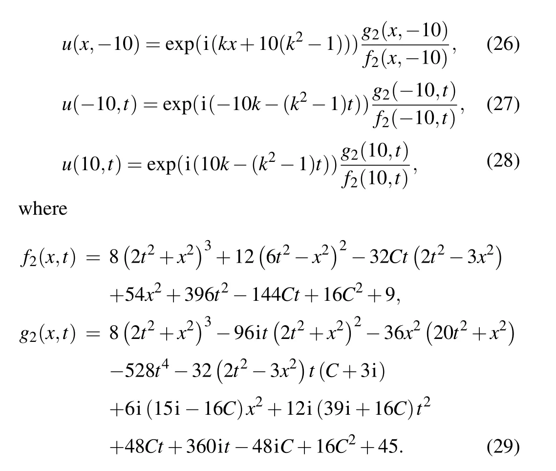
In the above equation, the value ofCis 100.First, we construct a deep neural network that is with seven hidden layers and 64 neurons in each hidden layer.During the training process, the learnable optimizer is still utilized to optimize the loss function,and the constants of the optimizer are set toλj=10-4.In addition, we still use the initial conditions as special Dirichlet boundary conditions on the spatio-temporal domain.The number of observations in this experiment is 400,and 20000 collocation points were selected for the construction of the differential equation constraints, and 400 sample points were selected for the initial condition constraints and boundary condition constraints.Figure 10 compares the difference between the prediction results of the improved PINNs and the true solution, from which we find that the improved PINNs obtain prediction results close to the true solution.Figure 11 shows the comparison between the prediction results of the improved PINNs and the true solution at different moments, and again we can find a high consistency between the two.Similarly, we calculate the L2 norm relative error of the prediction results of the improved PINNs with respect to the true solution, which has a value of 7.10×10-4, whilethe L2 norm relative error of the original PINNs with the same experimental setup is 7.49×10-3,and the results of the comparison are given in Fig.12.Also analyzing the computational efficiency,the time required for the improved PINNs to complete the training is only 59.3% of the training time of the original PINNs.In this study, we have also taken different numbers of neural network layers, neurons, and collocation points as variables, and analyze the effects of these variables on the prediction solution of second-order rogue waves for the nonlinear Schrödinger equation.In the specific experiments,we select different numbers of neural network layers,neurons,and collocation points for numerical experiments and compare the prediction solution errors of the original PINNs and the improved PINNs.The specific experimental results are shown in Table 3.Analyzing the experimental results, we can get the conclusion consistent with the previous experiments that with the increase of the number of neural network layers,the number of neurons,and the number of collocation points,the prediction solution error is also reduced.The experiment again demonstrates that for the second-order rogue wave prediction problem of the nonlinear Schrödinger equation,the improved PINNs outperform the original PINNs in terms of both computational efficiency and prediction accuracy.

Table 3.For the second-order rogue wave of the nonlinear Schrödinger equation,the errors of the predicted solutions are compared at different numbers of the neural network layers,different numbers of neurons,and different numbers of collocation points.

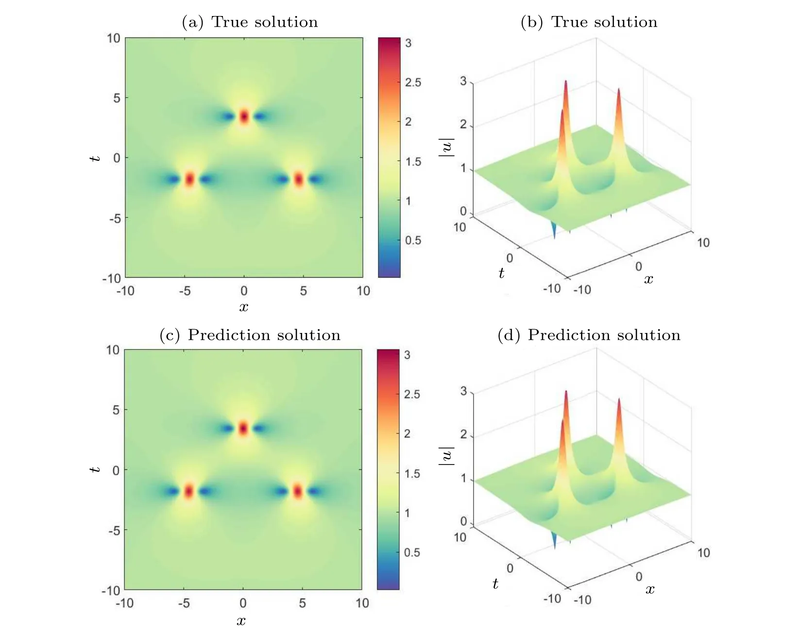
Fig.10.Exact second-order rogue wave solutions and predicted solutions of the nonlinear Schrödinger equation: (a)two-dimensional visualization of the true solution, (b)three-dimensional visualization of the true solution, (c)two-dimensional visualization of the predicted solution of the improved PINNs,(d)three-dimensional visualization of the predicted solution of the improved PINNs.

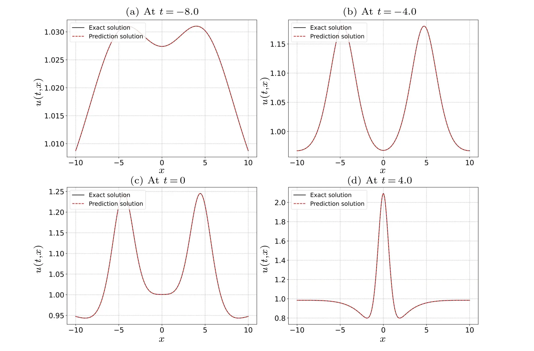
Fig.11.Comparison of the exact second-order rogue wave solution to the predicted second-order rogue wave solution of the nonlinear Schrödinger equation at four different time instances: (a)t=-8.0,(b)t=-4.0,(c)t=0.0,and(d)t=4.0.

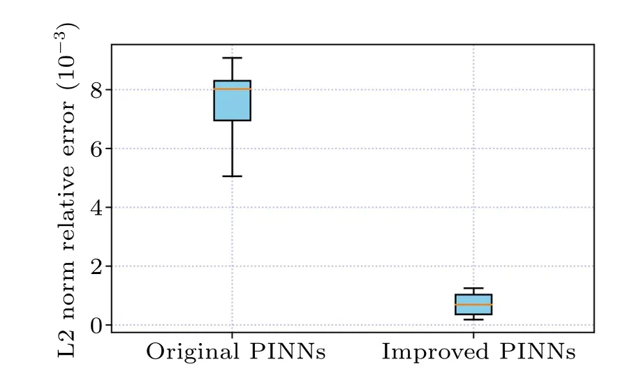
Fig.12.Visual analysis of errors in the prediction results of the secondorder rogue wave solution of the nonlinear Schrödinger equation: comparison of the errors of the improved PINNs and the original PINNs.

4.Conclusion

We have employed gradient-enhanced physics-informed neural networks(PINNs)with meta-learned optimization techniques for conducting numerical simulations of solitary waves and rogue waves.The enhanced PINNs incorporate gradient information, while the meta-learned optimization techniques significantly accelerate the training process of PINNs.As a result, the improved PINN model effectively harnesses more comprehensive physical insights and showcases superior generalization capabilities.Our experimental endeavors encompass the prediction of soliton solutions for the KK equation and rogue wave solution of the nonlinear Schrödinger equation using these enhanced PINNs, followed by a comprehensive evaluation of the predictive outcomes.Notably, our experimental results clearly show that the training speed of these improved PINNs is greatly improved,while the prediction error is significantly reduced.This overall enhancement substantially elevates the accuracy and efficiency of solitary wave and rogue wave simulations.Given the enhanced capacity of PINNs to simulate solitary wave and rogue wave phenomena,our future research endeavors are aimed at extending their applicability to other intricate system simulations.These include ocean mesoscale eddy simulations,typhoon simulations,and atmospheric turbulence simulations, among others.Furthermore, we will explore the integration of PINNs with pretrained language models to further investigate the potential of its application in the field of complex physics simulation and to extend its application to physics problems at various scales.

Acknowledgment

Project supported by the National Natural Science Foundation of China(Grant Nos.42005003 and 41475094).