Differences between two methods to derive a nonlinear Schrödinger equation and their application scopes

Yu-Xi Chen(陈羽西), Heng Zhang(张恒), and Wen-Shan Duan(段文山)

College of Physics and Electronic Engineering,Northwest Normal University,Lanzhou 730070,China

Keywords: dusty plasmas,nonlinear waves,particle-in-cell simulation

1.Introduction

Wave phenomena are a very common physical phenomenon that exist in many different systems, ranging from microscopic to macroscopic scales, from molecules to astronomical bodies.[1–6]Typical examples include plasma waves,[7–23]optical communications,[24–27]collective motion of particles in granular matter,[28,29]optical and acoustic wave phenomena in Bose–Einstein condensates,[30–36]etc.

Wave phenomena can be divided into two types: linear waves and nonlinear waves.The nonlinear waves usually can be approximately described by KdV equation[37–43]and NLSE.[44–50]These two equations can describe many different types of nonlinear wave phenomena.

It is worth noting that there are multiple methods available to obtain NLSE, such as the reductive perturbation method,[51–53]Krylov–Bogoliubov–Mitropolsky (KBM)method,[54–56]canonical transformation method,[57]inverse scattering transform method,[58]and so on.

The present paper is focused on two different methods to obtain the NLSE:One is to indirectly derive the NLSE,which is first to derive a KdV equation and then derive the NLSE step by step from the KdV equation,[59–64]while the other is to directly derive the NLSE from the original equation.[44–50,65,66]Although both methods can describe nonlinear waves, it is currently unknown whether the nonlinear waves described by these two methods are the same and which method is more accurate.Therefore,this is a problem that requires further study.

We investigated this problem based on dusty plasma and obtained the following results: First, the dispersion relation and group velocity of the envelope waves obtained by the two methods are different.Second,we used PIC numerical simulation method[67–74]to verify the two methods and found that both methods are correct for small amplitude envelope waves.Third, we investigated the dependence of wave amplitude on the perturbation parameterεε′for the first method and the dependence of wave amplitude on the perturbation parameterεfor the second method.The perturbation parameterε′actually stands for the quantity of ˜fd/fd0,where ˜fdrepresents the perturbed amplitude of the perturbations, whilefd0represent its corresponding amplitude at equilibrium state.For small amplitude, ˜fd/fd0is small enough, i.e.,ε′is small enough.The parameterεactually stands for the quantity ofλD/λ,whereλDrepresent the Debye length,whileλrepresents the wavelength of the envelope waves.For long wave length approximation,εis small enough.[70,73–76]Our results show that as the perturbation parameters increases,the envelope waves amplitude gradually increases.In addition, we found that as the envelope wave amplitude increases,the deviation between numerical and analytical results gradually increases.We determined the applicable scope of each method based on the deviation between numerical and analytical results and found that the method of directly deriving NLSE from the original equations has a wider applicable scope than that of step-by-step deriving NLSE from KdV equation.Lastly,we investigated the dependence of envelope width on wave amplitude numerically and analytically.

2.Theoretical model

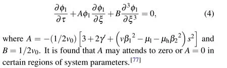
We now study dust acoustic waves in two-temperatureion dusty plasma which contain negatively charged dust particles, free electrons, and two different kinds of free ions.One kind of ions is high-temperature, while the other is lowtemperature.Charge neutrality condition at equilibrium isnil0+nih0=Zd0nd0+ne0, wherenα0is the number density of unperturbed particles of speciesα.α=il,ih,e,and d represent the low-temperature ion, the high-temperature ion, the free electron,and the dust particles,respectively.Zd0is the unperturbed number of charges residing on the dust grain measured in the unit of electron charge.Suppose that the dusty plasma is unmagnetized and collisionless.We now consider one-dimensional dust acoustic wave propagating in thexdirection.The dimensionless equations of motion of the system can be given as follows:[77]

wherendandudrefer to the number density and the velocity of dust fluid.φis the electrostatic potential.γ′=γTd/Zd0Teff.ne=νesβ1φ,nil=µle-sφ, andnih=µhe-sβ2φare the number densities of electrons,lower temperature ions,and higher temperature ions respectively,ν=ne0/(Zd0nd0),µl =nil0/(Zd0nd0),µh=nih0/(Zd0nd0),β1=Til/Te,β2=Til/Tih, ands= 1/(vβ1+µ1+µhβ2).Te,Til,Tih, andTdare the temperatures of the electrons, the low temperature ions,the high temperature ions,and the dust particles respectively.Teffis the effective temperature which satisfy 1/Teff=(ne0/Te+nil0/Til+nih0/Tih)/Zd0nd0.

All physical quantities in Eqs.(1)–(3) are normalized ones.They are normalized as follows:ndis normalized bynd0,nil,nih, andneare all byZd0nd0,ZdbyZd0,xby the Debye lengthλD=(kBε0Teff/nd0Zd0e2)2,tby the inverse of dust plasma frequencyω-1=(ε0md/nd0Zd02e2)1/2,udby the dust-acoustic speedcd=(kBzd0Teff/md)1/2,φbykBTeff/e,kBis boltzmann constant,ε0is vacuum permittivity.[77]

3.Derivation of NLSE for the system

To study nonlinear waves in a nonlinear system, two main methods are commonly used.One is to derive a KdV equation for localized waves using the reductive perturbation technique in the limit of small but finite amplitude and long wavelength.[37–43]The other method is to derive an NLSE when there are background waves present.[44–50]

There are also two different methods to derive an NLSE.One method involves first deriving a KdV equation and then obtaining an NLSE from the KdV equation.[59–64]The other method is to derive the NLSE from the original equation of motion,[44–50,65,66]for example, by obtaining an NLSE from hydrodynamical equations.A fundamental question is whether the NLSE and its solutions obtained from these two different methods are the same, and which one is more accurate.This paper aims to address these questions.

3.1.Derivation of NLSE from the CKdV equation

In this section, we will derive the NLSE from a coupled KdV (CKdV) equation for this system.Then we will compare its solutions with numerical results.Additionally,we will discuss the application scope of the analytical solution.

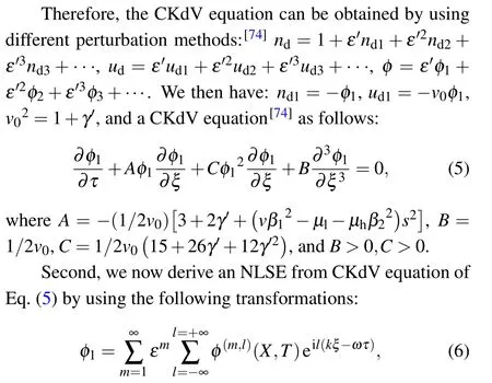
First, we derive a CKdV equation.By using the following expansionsξ=ε′(x-v0t),τ=ε′3t,nd=1+ε′2nd1+ε′4nd2+···,ud=ε′2ud1+ε′4ud2+···,andφ=ε′2φ1+ε′4φ2+···,whereε′is a small parameter,v0is the velocity of the dust acoustic KdV solitary waves.We then can obtainnd1=-φ1,ud1=-v0φ1,v02=1+γ′,and the KdV equation

Generally,we can use the KdV equation to approximately describe nonlinear waves in dusty plasmas.However, when the coefficients in the KdV equation are zero, the equation is no longer applicable.To address this specific condition of nonlinear wave behavior, we derived a new equation called the CKdV equation.The CKdV equation is an extension of the KdV equation that overcomes the limitation of zero coefficients.These coefficients can be tuned according to specific physical conditions, allowing the CKdV equation to more accurately describe the nonlinear wave in dusty plasmas,including phenomena that cannot be covered by the KdV equation.[77]whereX=ε(ξ-Vτ),T=ε2τ,Vis the group velocity.Substituting Eq.(6)into the CKdV equation of Eq.(5),we obtain the dispersion relationω=-Bk3,group velocityV=-3Bk2,φ(1,0)=0,φ(1,l)=0 for|l|>1,φ(2,2)=(A/6Bk2)[φ(1,1)]2,φ(2,0)=(A/V)|φ(1,1)|2and NLSE as follows:

whereP=-3Bk,Q=(A2/6Bk)-Ck.For an NLSE, whenPQ>0, the equation possesses bright envelope soliton solutions.Conversely,whenPQ<0,the equation possesses dark envelope soliton solutions.

In the present paper,we only consider the case ofPQ>0,i.e.,bright envelope soliton solutions.For this case,there are modulation instability which has been well studied in the previous investigations.[78–81]Therefore,in this paper,we do not do further research on modulation instability.Then,the envelope wave solution of Eq.(7)is as follows:

3.2.Derivation of NLSE from original hydrodynamical equations

In this section, we will use a different method for deriving the NLSE from the hydrodynamical equations given in Eqs.(1)–(3).We will also compare the numerical results with the analytical ones.Moreover, we will infer the application scope of the analytical solution.Later,we will also provide a comparison between the two methods employed for deriving the NLSE.

We use the following transformations

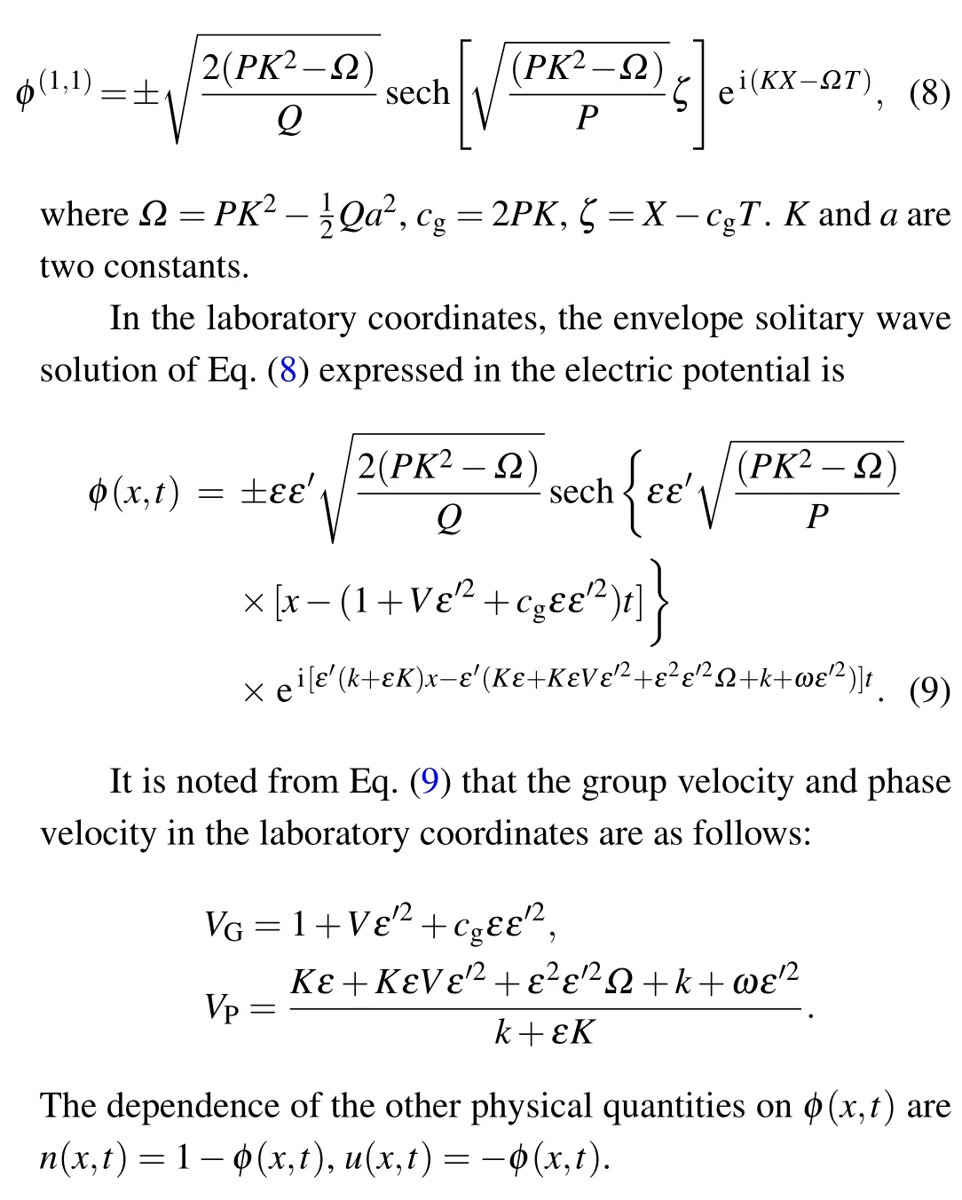
whereξ=ε(x-Vt),τ=ε2t,Vis the group velocity.Substituting these expansions into Eqs.(1)–(3), we haven(1,1)=-(k2/ω2)φ(1,1),u(1,1)=-(k/ω)φ(1,1),and the dispersion relationω2=k2/(k2+1),n(1,l)=u(1,l)=φ(1,l)=0 when|l|>1,n(1,0)=u(1,0)=φ(1,0)=0,the group velocity

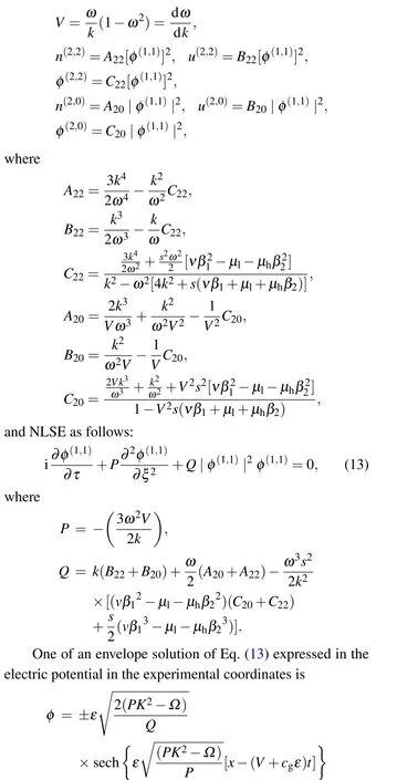
It is noted from Eq.(14)that the group velocity and phase velocity expressions in the laboratory coordinates are as follows:VG=V+cgε,VP=(ω+εKV+ε2Ω)/(k+εK).Relations among physical quantities aren=1-(k2/ω2)φ(x,t),u=-(k/ω)φ(x,t).

4.Comparisons between two different envelope waves obtained from two different methods

We have obtained two different expressions for envelope nonlinear waves, given by Eqs.(9) and (14), which were obtained from two different methods.One method involved first deriving a CKdV equation and then obtaining the NLSE,while the other method involved directly obtaining the NLSE from the hydrodynamical equations.

In this section, we will compare the differences between the two solutions and identify the differences.Additionally,we will determine the application scope of the two methods.

4.1.Comparisons the dispersion relation and the group velocity of the two methods

Firstly,in order to understand the differences in the envelope waves obtained from the two methods,we compared the dispersion relation and the group velocity of the two methods in Figs.1(a)and 1(b),respectively.

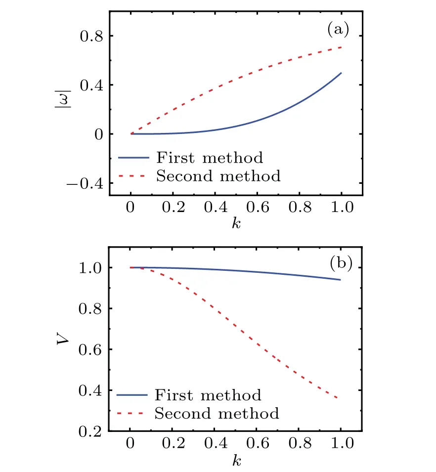
Fig.1.(a) The dispersion relation obtained from two different methods.(b) The group velocity of the envelope wave obtained from two methods.

As shown in Fig.1,two different methods have significant different behaviors for dispersion relation and group velocity.The wave frequency of the envelope wave obtained by the first method is smaller than that obtained by the second method for the same wave number.Moreover, the frequencies increase with the increase of the wave number.The group velocity of the envelope wave obtained by the first method is larger than that obtained by the second method for the same wave number.These results suggest that the envelope wave obtained by the two methods are significantly different.The purpose of the present paper is to verify the correctness of these two different methods.If both the two methods are correct, we will further compare the two methods and determine their respective application scope.

4.2.Comparisons the numerical results and the analytical result between two methods

In this section, we aim to compare the differences between the two solutions using the PIC numerical method,and then determine the application scope of each solution.

4.2.1.Particle-in-cell method

Particle-in-cell (PIC) simulation is commonly used for numerical work in plasma physics and particle dynamics because it provides an effective way to model the behavior of charged particles in a self-consistent electromagnetic field.PIC simulations are particularly well-suited for studying phenomena such as plasma waves,particle acceleration,and interactions between particles and fields.So, we use PIC method to simulate the envelope waves in this paper.

During the simulation process, the dust grains are represented by a limited number of “super-particles” (SPs), while both electrons and ions are treated as Boltzmann-distributed fluids.Each SP is assigned a weight factor, denoted byS,which represents the number of real particles it represents.Initially, the SPs are uniformly distributed in the simulation space,and their initial weight parameters S and velocities are determined from the initial conditions.[69,70]

To carry out the simulation,the simulation region is partitioned into several grid cells using the PIC method.As the dust particles move along their trajectories,they constantly exchange information with the background grid.At each time step,the positions and velocities of the SPs are weighted to all the grids,allowing for the calculation of the charge densityρg(or electric current densityJg).Once the charge densityρgis obtained, numerical solutions of either Maxwell’s equations(for the electromagnetic model) or the Poisson–Boltzmann equation (for the electrostatic model) are used to derive the electric field at each grid.In the electrostatic model,the magnetic field is assumed to be zero.[71–73]

Subsequently,the electric field imposed on each SP is determined, driving each SP according to Newton’s equation.This equation can be numerically solved using the leap-frog algorithm.Finally,the new positions and velocities of each SP are determined,and the simulation process repeats until completion.The summary of a computational cycle of the PIC method is shown in Fig.2.[71,72]

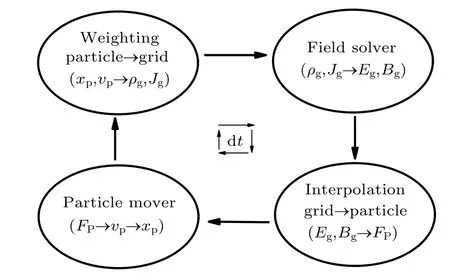
Fig.2.The summary of a computational cycle of the PIC method.

4.2.2.The initial conditions for the numerical simulation of the envelope wave

The simulation parameters we use are as follows:the spatial step is ∆x=0.5, the time step is ∆t=0.01, the number of grid cells isNx= 30000, the number of super particles contained in per cell is 100, the total length of thexaxis isLx=∆xNx,x0=3000.We choose periodic boundary conditions.The other parameters areTe= 5 eV,Til= 0.3 eV,Tih=5 eV,Td=200 K,Zd0=1000,nd0=1.0×1012m-3,nil0=1.0×1014m-3,nih0=1.0×1015m-3,k=0.1,K=0.1,a=1.

The initial conditions of the first method are given from Eq.(9)as follows:

The initial conditions of the second method are given from Eq.(14)as follows:

4.2.3.Comparisons between two methods

Figure 3 displays the envelope wave obtained by the first method at different timetthrough PIC numerical simulations.The numerical results exhibit excellent agreement with the analytical solutions derived from Eq.(9),as shown in Fig.4.

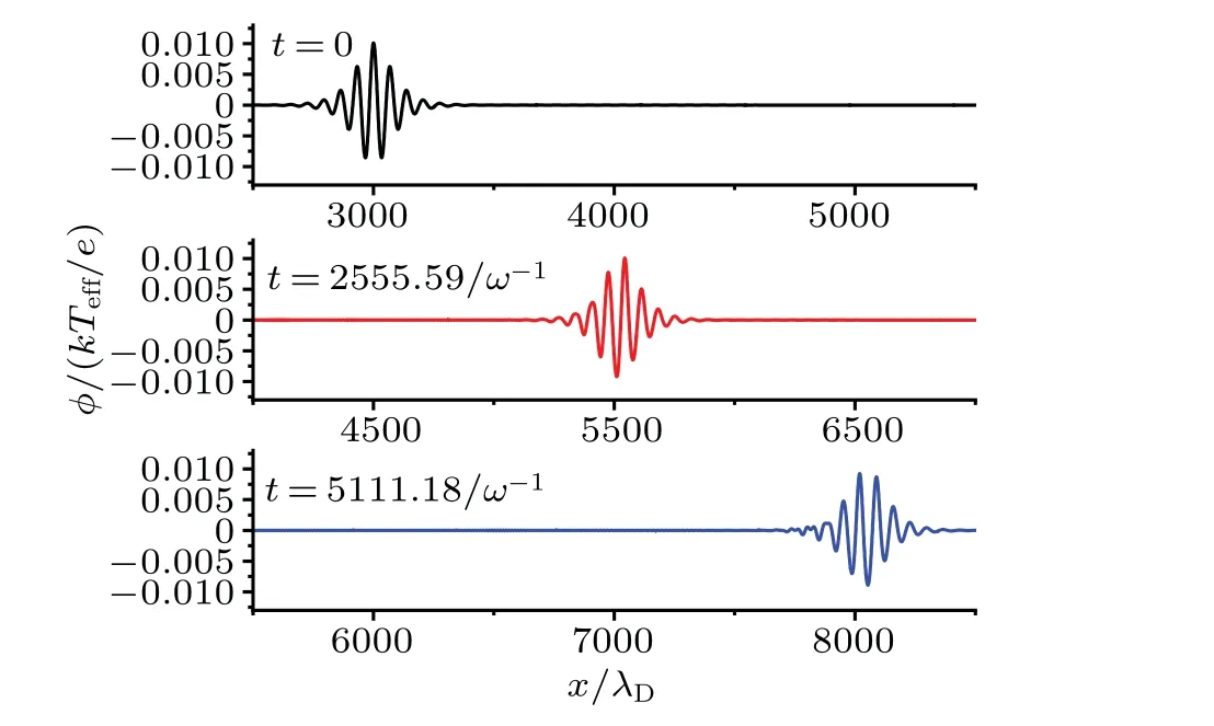
Fig.3.The PIC simulation results of the first method at different time t=0,t=2555.59/ω-1,t=5111.18/ω-1,where εε′=0.01,A=0.37.

Likewise,the numerical results of the envelope wave obtained by the second method at different timetis shown in Fig.5.The numerical results obtained through PIC simulations also show good agreement with the analytical solutions derived from Eq.(14),as depicted in Fig.6.

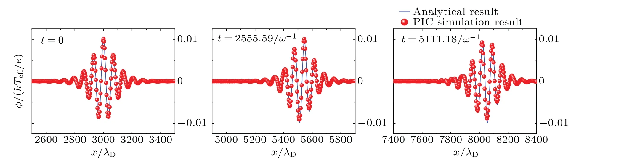
Fig.4.The comparisons between PIC simulation results and the analytical ones of the first method at different time t =0,t =2555.59/ω-1,t=5111.18/ω-1,where εε′=0.01,A=0.37.

It is evident from Figs.3 and 4 that the analytical result of the envelope wave obtained by the first method seems valid,as the numerical results show that it can propagate stably.This suggests that the NLSE obtained by the first method is correct.Similarly,figures 5 and 6 indicate that the analytical result of the envelope wave obtained by the second method is also valid,and therefore,the NLSE obtained by the second method is correct as well.

While figures 4 and 6 show good agreement between the numerical and analytical results for both methods, it is unclear if this agreement holds for larger amplitude (φm) envelope waves.In order to understand it,we compare the numerical results with that of the analytical ones for larger amplitude waves for both cases by varying the parameter ofεsinceεindirectly stands for the wave amplitude (It is noted from Eqs.(9) and (11) that the amplitudes of the envelope waves contain the parameter ofε), while keeping the other parameters constants.

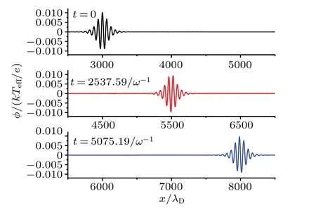
Fig.5.The PIC simulation results of the second method at different time t=0,t=2537.59/ω-1,t=5075.19/ω-1,where ε =0.01.

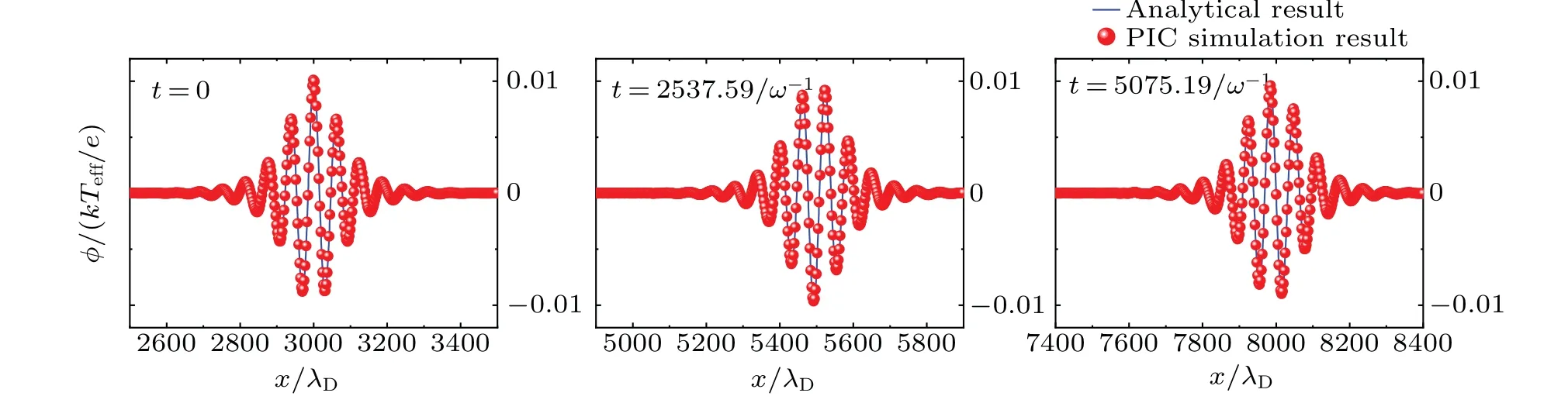
Fig.6.The comparisons between PIC simulation results and the analytical ones of the second method at different time t=0,t=2537.59/ω-1,t=5075.19/ω-1,where ε =0.01.

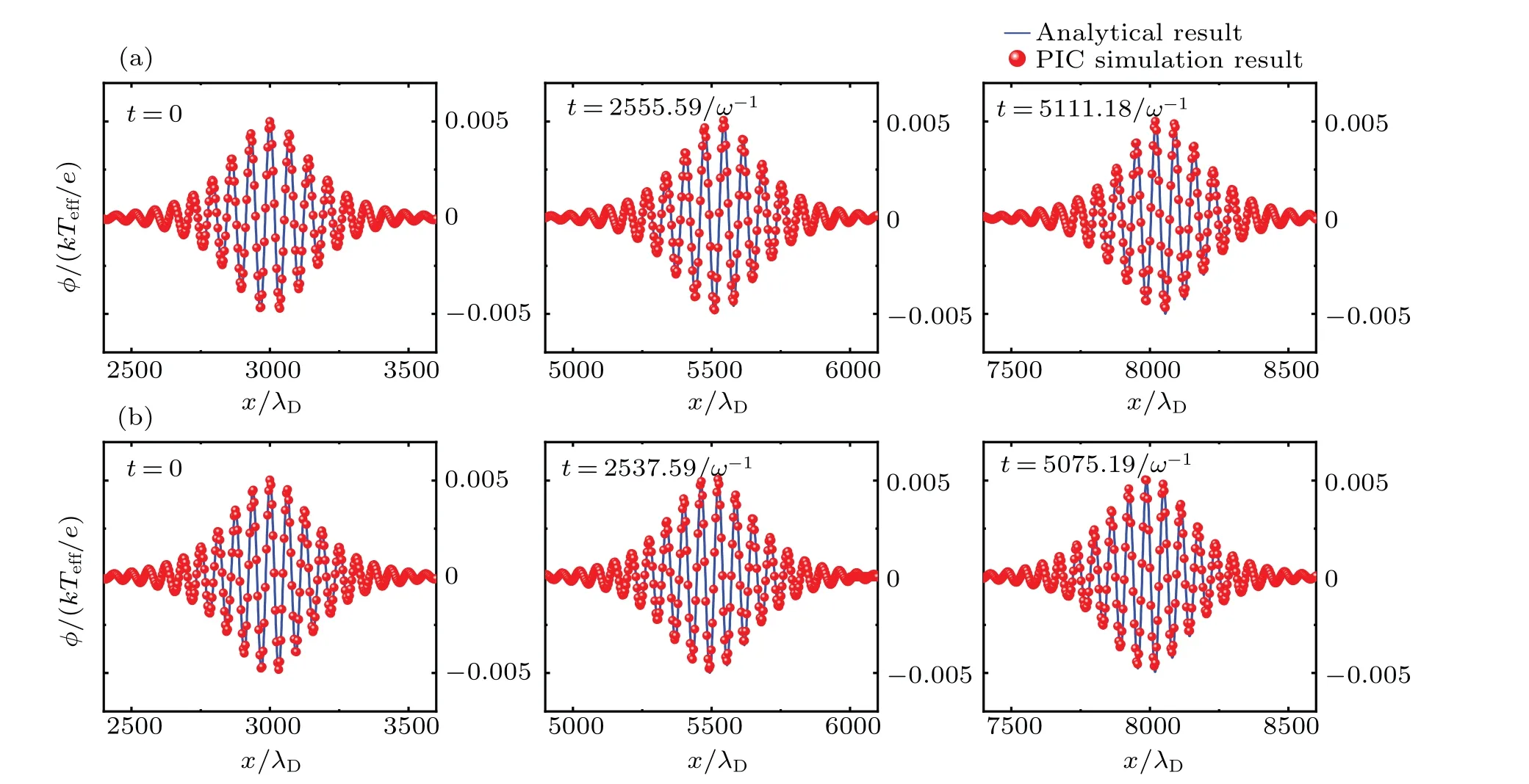
Fig.7.The comparisons between PIC simulation results and the analytical ones at different time t,where φm=0.005.(a)The result of the first method.(b)The result of the second method.

The waveforms for the numerical and analytical results of the different amplitude envelope waves at different time for two different methods are shown in Figs.7 (φm=0.005), 8(φm=0.015), and 9 (φm=0.025).By examining these figures, we can determine whether the numerical and analytical results are in good agreement for larger amplitude envelope waves.Notice from Figs.7 and 8 that both the numerical and analytical results are in good agreement for larger amplitude waves.However,in Fig.9,the difference between the numerical and analytical results is more obvious for both methods.It appears that as the amplitude of the envelope wave increases the differences between the numerical results and analytical ones become more pronounced.

To gain further insight into the differences between the PIC numerical results and the analytical ones for both methods,we present the dependence of the wave amplitude(φm)onεε′orεfor the two cases in Fig.11.It can be observed from Fig.11,that the amplitude of the envelope wave increases with increasing ofεε′orε.Asεε′orεincreases,i.e.,wave amplitude increases, the differences between the analytical results and the numerical ones obtained from both methods become larger.In other word, the analytical results are valid if the amplitude is small enough.Based on these results, the application scope of both methods can be determined from Fig.10.Specifically,the first method can be applied whenφm<0.01,while the second method can be applied whenφm<0.015.

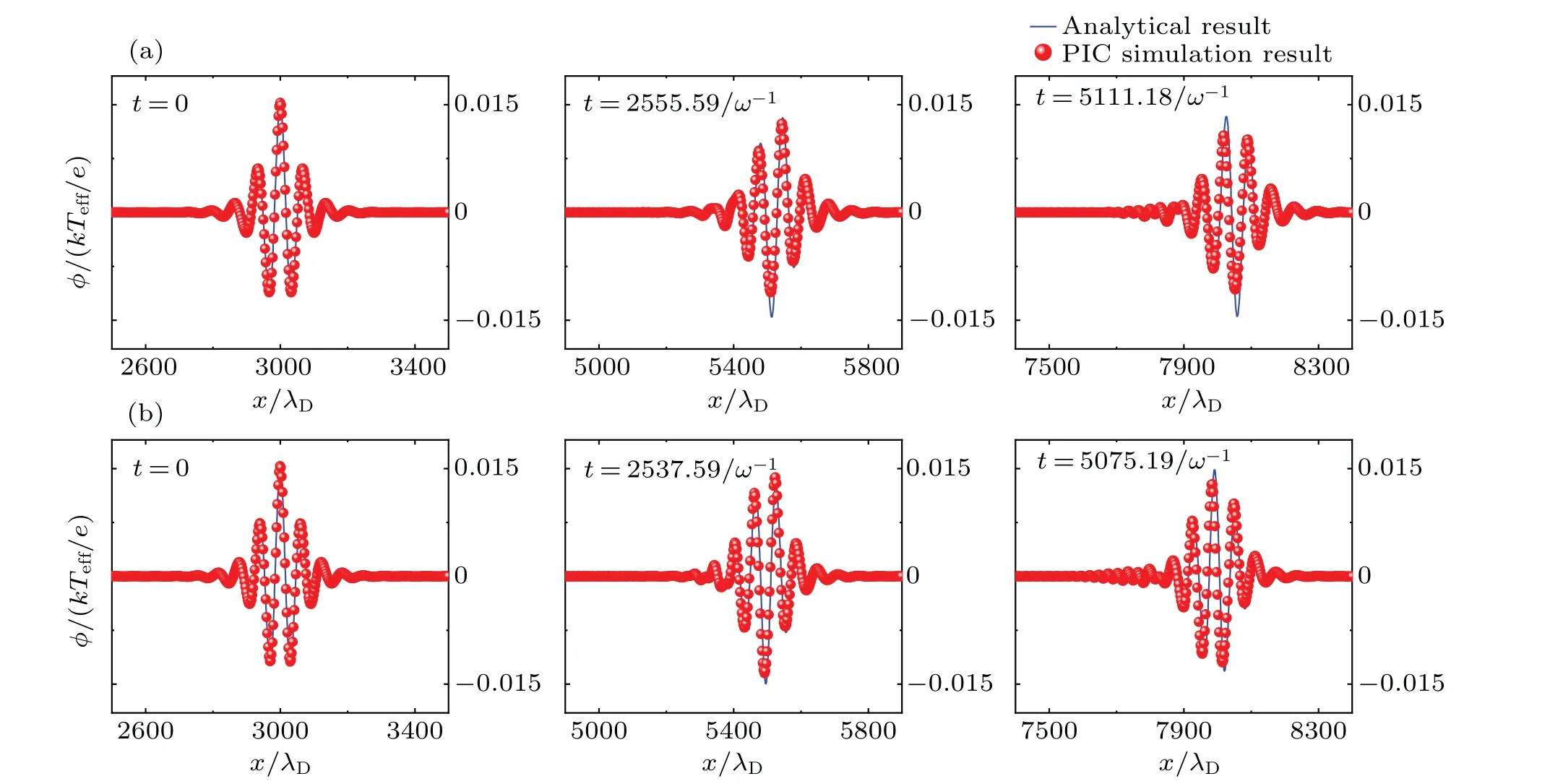
Fig.8.The comparisons between PIC simulation results and the analytical ones at different time t,where φm=0.015.(a)The result of the first method.(b)The result of the second method.

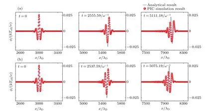
Fig.9.The comparisons between PIC simulation results and the analytical ones at different time t,where φm=0.025.(a)The result of the first method.(b)The result of the second method.

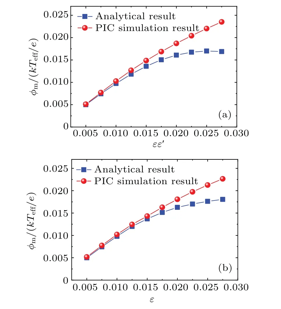
Fig.10.Comparisons between the numerical results and the analytical ones.(a)The dependence of the wave amplitude(φm)on the parameter εε′ for the first methods.(b) The dependence of the wave amplitude(φm)on the parameter ε for the second methods.

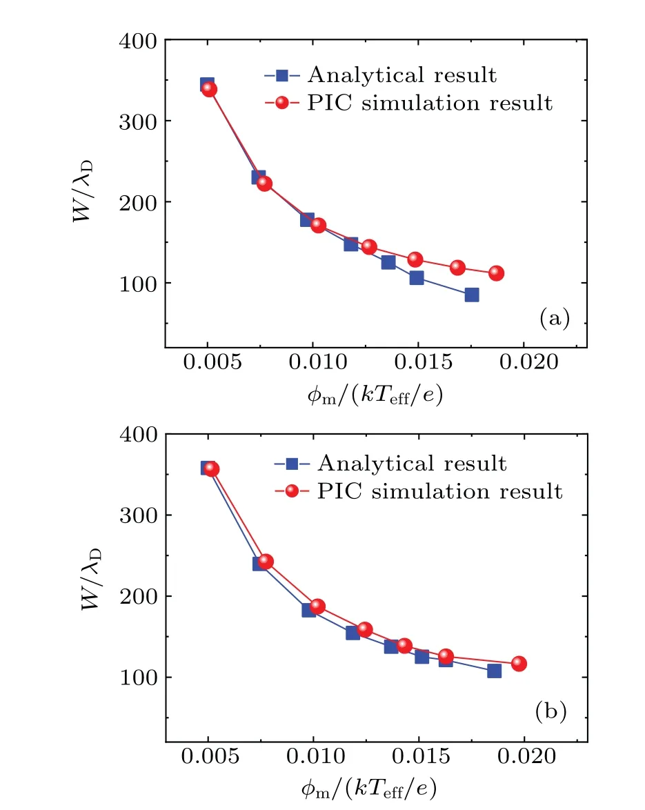
Fig.11.Comparisons between the numerical results and the analytical ones of the dependence of the width of envelope waves on the wave amplitude: (a)for the first method and(b)for the second method.

To further understand the differences between the two methods, the dependence of the width of the envelope waves(W)on the wave amplitude(φm)is shown numerically and analytically in Fig.11.It seems from Fig.11 that the deviation of the wave width between the analytical results and the numerical ones of the first method is obvious when the wave amplitude is larger than 0.01, while the deviation of the second method is still not significant even when the wave amplitude is around 0.02.Therefore, the application scope of the envelope wave obtained from the second method is wider than that from the first method.

5.Discussion and conclusion

The present paper chooses a dusty plasma as an example to numerically and analytically study the differences between two different methods of obtaining NLSE.It is found that the envelope waves from the two methods have different dispersion relations, different group velocities.Specifically,the wave frequency of the first method is lower than that of the second one for the same wave number,while the group velocity of the first method is larger than that of the second method for the same wave number.It is noted that the two methods are completely different.

Additionally, the application scopes of two different methods are shown.The results indicate that the application scope of the envelope wave obtained from the second method is wider than that of the first method.It is suggest that both methods to derive NLSE are correct in the regime of their application scope.In other words, if the amplitude of the envelope solitary wave is smaller that a critical values(the critical values are different for two different methods), the analytical results are valuable to describe the real solutions of the envelopes waves.If the amplitude of the envelope solitary wave is larger than this critical value,the neglected higher order terms in deriving the NLSE play an important role which should not be neglected.

In conclusion,although both methods are valuable within the range of their respective application scopes,the two envelope wave solutions obtained from the two different methods are completely different.For other systems,both methods may also be used to derive the NLSE and obtain an envelope wave or other nonlinear waves such as Rogue waves,but their solutions are possibly different.

Acknowledgements

Project supported by the National Natural Science Foundation of China (Grant Nos.11965019 and 42004131) and the Foundation of Gansu Educational Committee (Grant No.2022QB-178).