Spatial search weighting information contained in cell velocity distribution

Yikai Ma(马一凯), Na Li(李娜), and Wei Chen(陈唯),‡

1State Key Laboratory of Surface Physics and Department of Physics,Fudan University,Shanghai 200438,China

2China National Center for Bioinformation,Beijing 100101,China

3National Genomics Data Center,Beijing Institute of Genomics,Chinese Academy of Sciences,Beijing 100101,China

Keywords: cell migration,foraging efficiency,random walk,spatial search weight

1.Introduction

Cell migration is a topic of significant interest in the fields of biology, medicine, and physics.[1–3]Physicists primarily study cell migration behavior using methods such as generalized Langevin equations and models of nonlinear dynamics.[4–9]It is evident that the random walk of cells differs significantly from the passive walk of particles driven by thermal fluctuations,as observed in the mean square displacement and probability distribution of cell velocities.[8,10–13]It is a natural idea that the migration behavior of organisms may be related to their efficiency in foraging and searching.Therefore, researchers have conducted numerous studies on the relationship between biological movement patterns and search efficiency.[14–18]However,the majority of studies in this field have primarily focused on individual trajectory characteristics.There is a relative scarcity of research examining the relationship between collective characteristics of biological group movement and foraging efficiency.We noticed that there are significant differences in the average trajectory velocities of individual cells,[19]implies that cells within a community exhibit variability.In this paper,we aim to explore how the distribution ratio of high-speed cells and low-speed cells in such cell communities affects the foraging efficiency of the cell community.Our work indicates that,through considering weights of spatial search, the experimentally obtained velocity distribution corresponds to an optimal search strategy.We speculate that this specific spatial search weighting is an evolutionary outcome associated with the historical survival environment,ultimately manifested in the distribution of cell velocities.

The article is organized as follows: Firstly, Section 2 presents the experimental methods and results.Then, in Section 3, a simulation model is established based on the experimental data.Next, Section 4 calculates the search efficiency under different cell speed distributions using the established framework, and Section 5 discusses the results.Section 6 introduces spatial search weights as a model improvement.Subsequently, Section 7 recalculates the search efficiency within the updated model, and Section 8 provides a comprehensive analysis of the results.Finally,Section 9 summarizes the findings and contributions of the study.

2.Experimental results

Dictyostelium discoideum cells(Dicty)were used as the model cells for our study.The methods used for preparing Dicty cells and acquiring data are similar to those described in Ref.[20].In the experiment,starving KAx-3 Dicty cells were dispersed onto nutrient-free agar surfaces after a 2-hour starvation period in 5◦C.The planting density is 30 cells/mm2,and the samples were kept at room temperature throughout the entire observation period.In the absence of food, Dicty cells exhibit random movement on agar surfaces as they search for sustenance.The movement trajectories of cells were continuously captured using a microscope equipped with a digital camera (Olympus CX23, objective 4×; Canon EOS 100D).The images are captured with a spatial resolution 5184×3456 and a time interval ∆t=20 s.

We employed a home-made IDL program to track the positions of cells at each time, allowing us to obtain spatial trajectoriesr(t) of the cells.We quantified the spatial distance∆rtraveled by the cells during a given time interval ∆t.The instantaneous velocityvtof the cells was calculated using the formulavt=∆r/∆t.For each obtained cell trajectory,we can define the trajectory velocityvof the cell using

Here,the timeTrepresents the time duration of the cell movement trajectory.The difference betweenvandvtlies in the following: the difference invtrepresents the instantaneous fluctuations in the velocity of individual cells,while the difference invrepresents the inherent velocity differences among different cells observed in the cell community.Based on the calculatedvfrom different cell trajectories,we can calculate the number of cells with different trajectory velocitiesvin the cell community, and accordingly, plot the probability density distribution curveP(v), which represents the proportion of cells with different trajectory velocityvin the cell community.TheP(v)curve is depicted in Fig.1.

From Fig.1, it shows that within the same cell colony,cells spontaneously divide into subgroups with different speeds during their spatial search for food.The speeds of high-speed and low-speed cells can differ by an order of magnitude.The peak on the left side indicates that, in the Dicty cell colony, most cells have small velocities, and only a few cells are able to move quickly over long distances.

The shape of theP(v) curve resembles the Maxwell–Boltzmann distribution of an ideal gas.Therefore, we have developed a phenomenological model (Eq.(2)) based on the Boltzmann formula to describe the shape of theP(v)curve:

wherekis the normalization coefficient.From they-log plot of the curve,the insert in Fig.1,it is evident that the decrease in the high-speed segment follows a linear decay rather than a quadratic decay.Hence, the exponential term in Eq.(2) is expressed as exp(-v/v0) instead of exp(-(v/v0))2.When fitting the actual data,we discovered that the value ofαis approximately 2.Consequently, in subsequent fittings, we fixα= 2 and only adjustv0as the sole adjustable parameter.This approach provides an advantage in subsequent simulation work where we require a series of velocity distributions with continuous changes.By only modifying the parameterv0,we can achieve different widths of the distribution and most probable speeds ofP(v)curves.

Due to the noticeable discrepancy in cell velocities within the colony, we aim to comprehend the variations in random walking patterns exhibited by cells with varying velocities.To divide the cells into five groups according to their cell trajectory velocitiesv,we plotted mean square displacement(MSD)curves for these five cell groups.The results are shown in the following Fig.2.

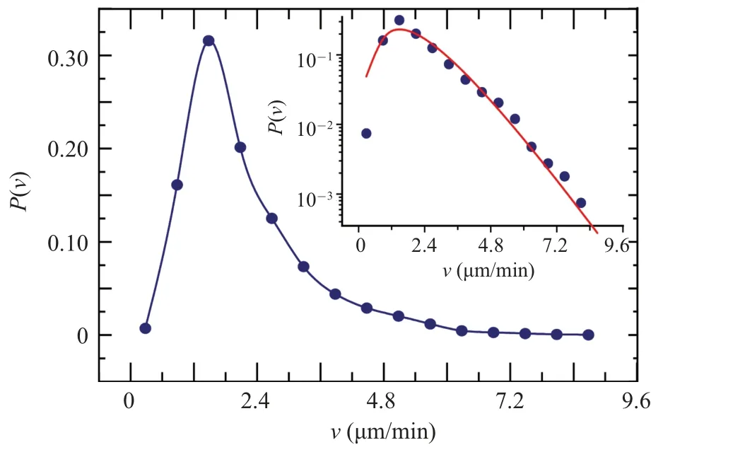
Fig.1.The distribution of Dicty cell trajectory velocities.The insert in the figure is presented in a y-logarithmic plot, and the red solid line represents the fitting line of Eq.(2)with the fitting parameter value v0=0.72µm/min.

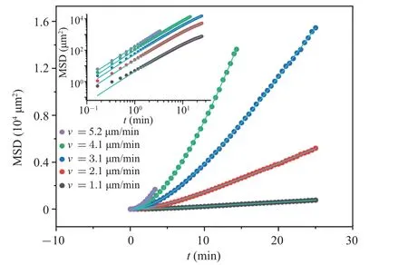
Fig.2.The variation of〈r2〉(MSD)with time t for 5 groups of cells with different trajectory velocities v(dots).From bottom to top,each curve corresponds to velocity groups v=1.1±0.2, 2.1±0.2, 3.1±0.3, 4.1±0.4,5.2±0.6 µm/min.The solid line represents the fitting line of Eq.(3), and the fitting parameter values for each curve are listed in Table 1.

Many papers have discussed the difference between the〈r2〉of Dicty cells and Eq.(3).[8,10]In our results, all the fitted curves and experimental data agree well, except for the〈r2〉curve corresponding to the lowest speed that exhibits noticeable deviations in the short-range limit.Therefore, we consider Eq.(3) as a first-order approximation that adequately captures the essential characteristics of random cell movement in our experiments.The primary advantage of using Eq.(3)is its ability to directly derive the two critical characteristics of random walking behavior: persistent timeτand diffusion coefficientD.Persistent timeτrepresents the duration during which cell movement tends to be in a straight line,or,in other words, the time it takes to forget the initial movement direction.The fitting results of the parametersτandDfor each〈r2〉curve are listed in Table 1.

Table 1.The persistent time τ and diffusion coefficient D for each group of cells with different trajectory velocities v.

Table 1 illustrates the distinction in walking patterns among various cells.It can be observed that as the trajectory speedvof cells increases, the diffusion coefficientDalso increases correspondingly.The persistent timeτof the cells follows a similar trend, except for a slight deviation inτfor the last group(with a cell proportion of less than 8%).

To have a more intuitive understanding of the diffusion speed and turning frequency of cell groups with different speeds, figure 3 shows the trajectory of different-speed cell groups.The highest velocity we measured was approximately 9.2 µm/min.Hence, we divided the velocity into three categories on the trajectory plot:(0–3),(3–6),(>6)µm/min.Figure 3 provides a visual representation of this correlation.It illustrates that highly mobile cells exhibit trajectories with long persistent length,characterized by a longer persistent time(τ)and are represented by green trajectories.On the other hand,cells with a slower speed of movement display more curved and coiled trajectories, which are represented by trajectories with smaller persistent times(τ).By combining the information from Table 1 and Fig.3,we can conclude that cell velocities represented correspond to specific motion models(v,τ,D)indeed.

3.Problem presentation and model approach

The cell colony originates from a single spore.Why do they exhibit different distributions of motion patterns(v,τ,D)instead of sharing a single motion pattern? We consider that cell movement is for food searching.Therefore, we hypothesize that cell colonies may move with specific motion patterns to maximize the spatial search efficiency of the entire cell colony.From Fig.3, it can be observed that high-speed cell movement covers a greater distance, but their trajectories are straighter and resulting in more blank spaces between them.On the other hand,low-speed cells have smaller persistent timeτand more curved trajectories, which fill in the blanks between high-speed cell trajectories.Intuitively, a combination of specific high and low-speed cells might be more favorable for cell spatial search.The observed cell speed distributionP(v) in our experiment may represent an optimized motion pattern for cell spatial search efficiency.

To validate our hypothesis, we developed a numerical model and utilized the framework of the OU process to simulate the movement trajectories of cell colonies.[21]The simulations considered different cell speed distributions represented byP(v), which corresponded to distinct motion patterns (v,τ,D) as indicated in Table 1.By examining these simulated movement trajectories,we could evaluate their spatial search efficiencies.By comparing the spatial search efficiencies of the cell colony trajectories associated with different speed distributionsP(v), we investigated whether the experimentally obtainedP(v)aligned with the highest spatial search efficiency.

4.Simulation model establishment

By continuously changing the value ofv0in Eq.(2), we can generate different velocity distributionsP(v),as shown in Fig.4.

From Fig.4, it can be observed that a smallerv0represents a smaller proportion of high-speed cells in the colony,while a largerv0represents a more even velocity distribution.Therefore,the velocityv0can be used as a characteristic quantity to describe theP(v)distribution.It is worthy to note that directly using the distribution generated by Eq.(2)would lead to a problem: different distributions correspond to different average velocities of the cell colony.Therefore, we need to truncate the highest velocity of theP(v) curve generated by Eq.(2),in order that the average velocity of the simulated cell colony remains unchanged.After this treatment, the normalizedP(v)result that satisfies velocity normalization andP(v)probability normalization is shown in Fig.4.

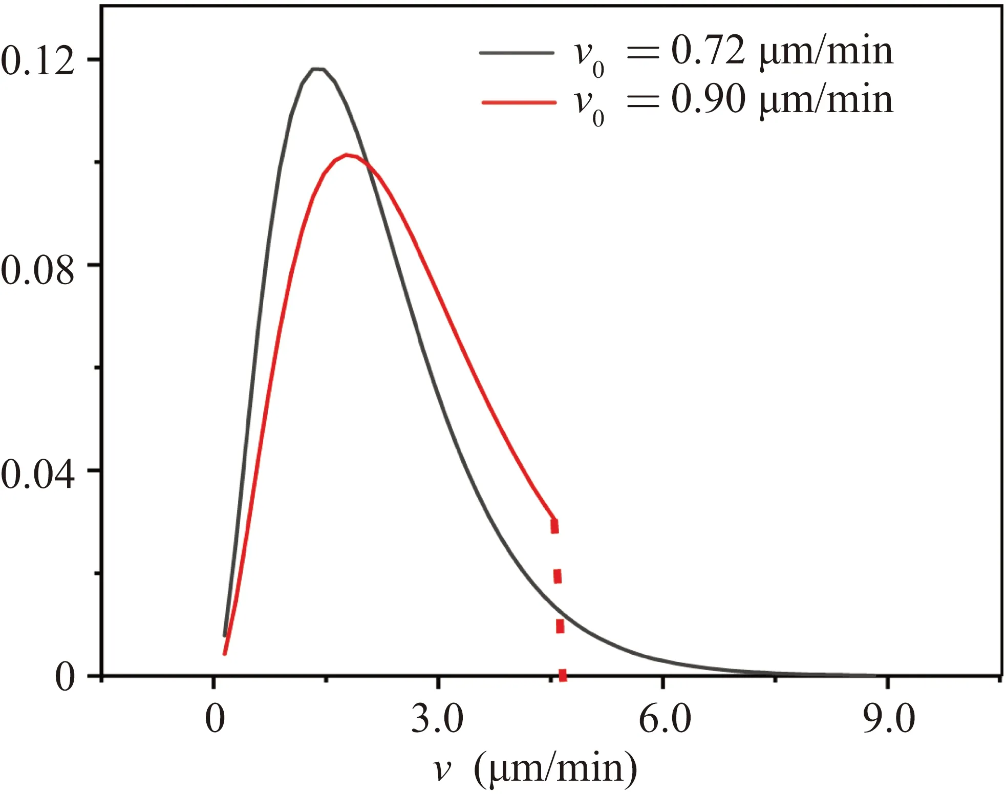
Fig.4.The result of velocity distribution curve P(v) after being normalized by average velocity.The left curve corresponds to v0 =0.72µm/min,and the right curve corresponds to v0=0.90µm/min.

We simulate a cell population to generate a specific velocity distribution curveP(v) based on the cell seeding density, cell diameter, and microscope field of view size used in our experiment.Periodic boundary condition is used to keep the total number of cells in the field of view constant.We use the OU process to simulate the motion trajectories of all cells,aiming to match the characteristic values(v,D,τ)of cell grouping with Table 1.The width of the cell trajectories was set to match the size of the cells.

Based on the simulation results, we obtained the celltrajectories images,as shown in Fig.5(a).

The cell trajectory images generated through simulation are presented in black and white format: the grayscale value of the area covered by the cell trajectories was set as 1 (representing the searched area),while the uncovered area was set as zero(representing the unsearched area).We utilized Eq.(4)to calculate the proportion of white regions in the image,represented asCR.

whereg(i)represents the grayscale value of eachipixel in the image, andArepresents the total number of pixels in the image.The relationship betweenCR, which represents the proportion of the area covered by cell trajectories,and the random walking timetis plotted in Fig.5(b).

Thus, we can define the search efficiency by the growth rate of theCR(t)curve.However,as seen from the fitted curve in Fig.5(b),CR(t)cannot be well fit to the exponential modely=1-exp(-t/t0).The difference between the fit and simulation results becomes more pronounced when dealing with higher cell density in experimental studies or larger cell size in simulations.Therefore, we cannot quantitatively measure the spatial search efficiency of the cell colony using the characteristic timet0of the exponential model.Hence,we directly defineE,the average value ofCRwithin the search timeTsas given in Eq.(5),as the characteristic value of the spatial search efficiency of the cell colony.

A larger value ofEindicates higher search efficiency.As shown in Fig.6,afterCR(t)reaches saturation,the monotonicity and overall trend ofEare not affected by the length of the search timeTs.Therefore,Ecan be considered as a reliable physical quantity to define the search efficiency.

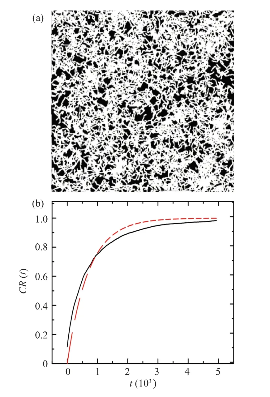
Fig.5.(a) Simulated cell motion trajectory graph, simulated for 5000 steps.(b)The relationship between the proportion of white area in the image CR and time t in panel(a).The black line represents the numerical calculation result of the image.The red dashed line represents the fitting curve of y=1-exp(-t/t0).

5.Discussion of the model results

Using the above method,we simulated the movement trajectories of cell colonies under differentP(v)distributions by continuously changing the values ofv0in Eq.(2)and obtained differentCR(t)curves as shown in Fig.6(a).The spatial search efficiencyEfor eachCR(t) curve is calculated according to Eq.(5).TheE(v0)curve is plotted in Fig.6(b).Among them,v0=0.72 µm/min corresponds to the velocity distribution of cells in the experiment.From Fig.6(b), it can be observed that the spatial search efficiencyEmonotonously varies withv0.[22]This is contrary to our initial expectation.

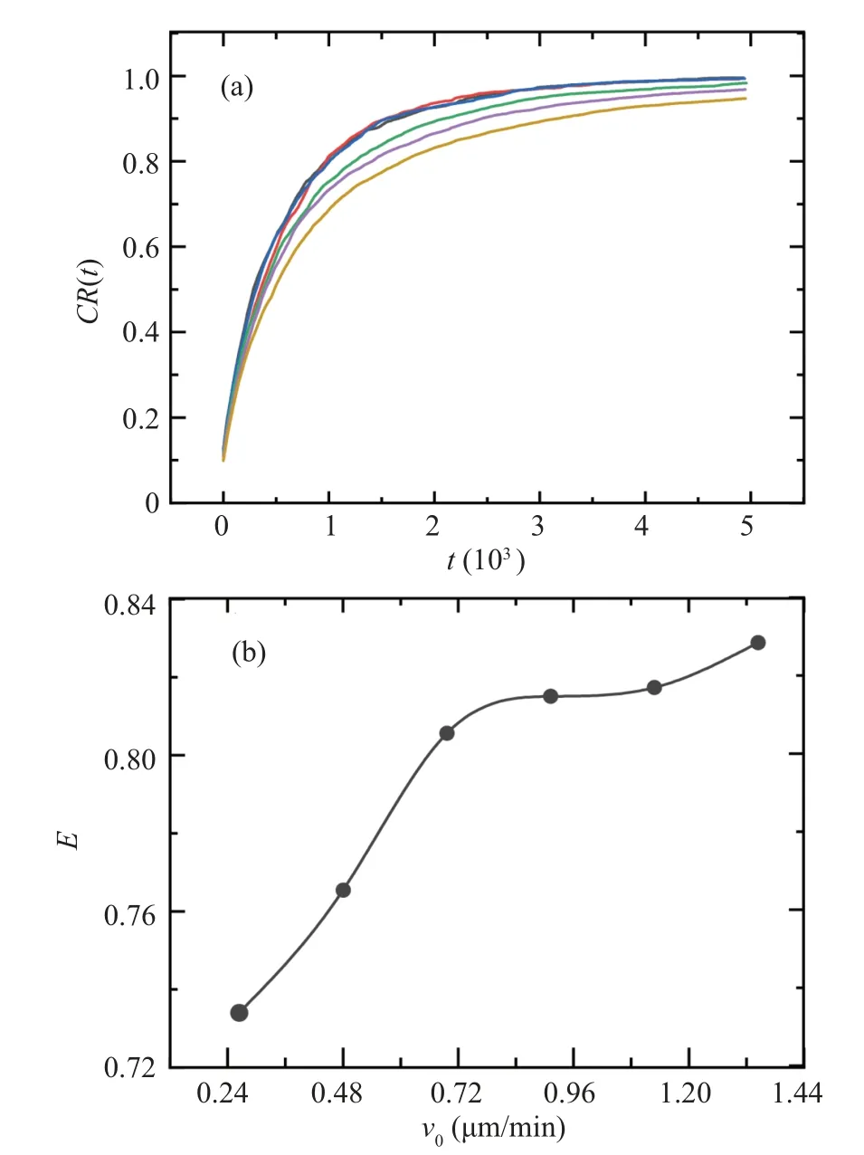
Fig.6.Simulation of spatial coverage ratio CR(t)derived from different P(v) distributions obtained from Eq.(2).From top to bottom, the curves correspond to v0 =0.24, 0.48, 0.72, 0.96, 1.20, 1.44 µm/min.(b)Relationship between cell spatial search efficiency E and v0.

Recalling our definition of spatial search efficiency, the monotonous increase inEis actually natural: the more highspeed cells there are, the more distance the cell colony naturally covers in the same time period.Therefore, more new areas are covered, which leads that the corresponding spatial search efficiency is higher.However,this does not align with our initial intuition.

Intuitively, we believe that the trajectory graph of cells moving in a straight line at high speeds may not necessarily be the optimal choice: because cells tend to move straight at high speeds,there are often many blank spaces between cell trajectories, which is not conducive to cell food search.However,in our previous model,an increased number of blank spaces in the movement trajectory does not affect the spatial search efficiency: the exploration of distant regions by high-speed cells compensates for those missed blanks in the nearby locations.But in the real world,the significance of search results at different distances is obviously different for cells.The distribution characteristics of food can significantly affect the search strategy of organisms.[23]Finding food closer to the colony is more meaningful for the bacterial population.However, our previous model did not take this into account.

6.Introduction of spatial search weights W(r)

As mentioned before,we need to consider the differences in spatial search weights corresponding to different positions in the cell movement trajectory in space,with higher weights in places closer to the initial distribution of the colony.Then we will construct a function to describe such a distribution of spatial weights.Considering that the spatial distribution range of cells is within the size range of cell spores,the spatial search weight for finding food within this region should be the highest and consistent,and then the weight should start to decrease gradually as the distance from the colony center increases.According to the above assumption,we construct the cell spatial search weight functionW(r) as given in Eq.(6).Here, we have not used a simple Gaussian distribution to consider that the spatial search weight within the initial spatial distribution region should be similar.

Here,ris the radial distance from the center of the cell colony.The parametersr0andrgcorrespond to the width of the equally weighted central region and the rate of weight decrease with distance,respectively.

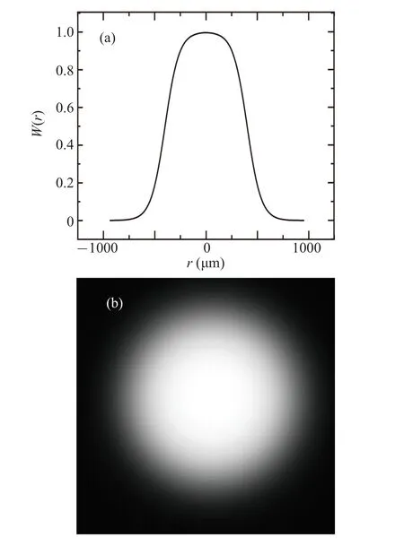
Fig.7.The cell spatial search weights calculated according to Eq.(6)for r0 = 600 and rg = 100, as well as their distribution in a twodimensional space(a)and with respect to the spatial distribution of the cell colony(b).The center point in panel(b)corresponds to the center of the spatial distribution of the cell colony.

According to Eq.(6),the distribution of cell spatial search weights is shown in Fig.7.We should multiply this weight distributionW(r)(Fig.7(b))with the image of the distribution trajectory of cells(Fig.5(a)).This will yield a new weighted trajectory image.

We simulate the cell motion trajectory again using the above method.Initially,the cells are distributed in a finite central area with a size ofr0and the periodic boundary conditions are removed.The motion trajectories of the cells are recalculated under differentv0(corresponding to differentP(v)).According to the weighted modified trajectory image obtained from each simulation, as shown in Fig.8, which is technically obtained by multiplying the trajectory map (similar to Fig.5(a)) by the spatial distribution (Fig.7(b)).The characteristic valueEof the current spatial search efficiency is recalculated.and we can recalculate the equivalent coverage rateCR(t)curve based on Eq.(4).At this time,the gray valueg(i)in Eq.(4)is just as we expected after being modified byW(r).

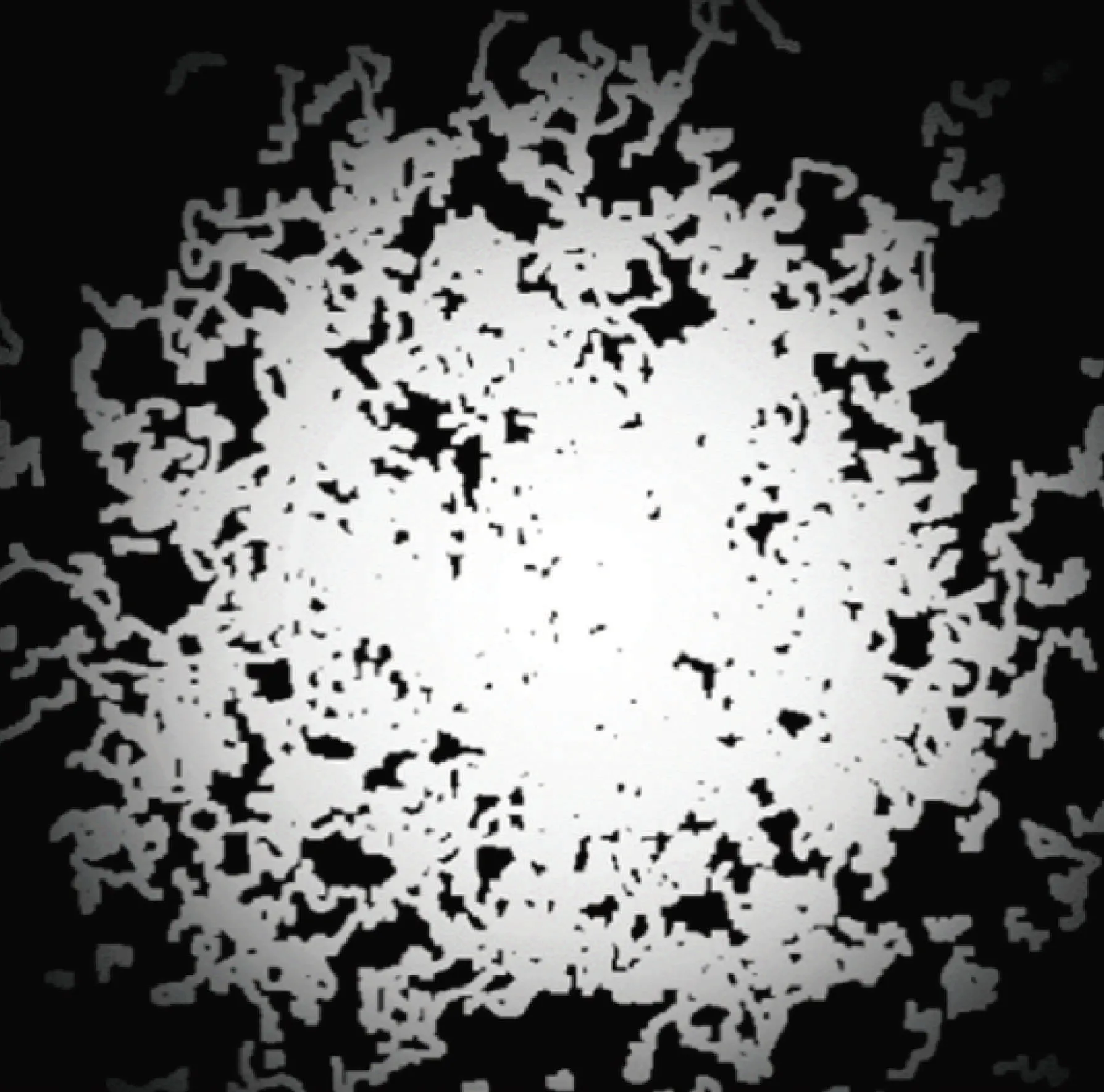
Fig.8.The modified cell trajectory map considering spatial search weight W(r).

The optimum spatial search efficiency corresponding to the black curve in Fig.9 is around 0.5µm/min.This does not matchv0=0.72µm/min(the fitted result of the experimental data).But this is natural because the form of ourW(r)is an arbitrary assumption.We do not know the specific form ofW(r)used by cells in the real world.The value ofrg=68 used in Eq.(6)is just an arbitrarily generated weight curve.The result of the black curve in Fig.9 only indicates that in our model,given a spatial search weight distributionW(r),there is indeed an optimal velocity distribution for a cell colony instead of a higher proportion of high-speed cells being better.

7.The spatial search efficiency E modified by W(r)

The simulation results show that under the limitation of spatial search weightW(r), the spatial search efficiencyEof cell colonies can indeed reach the maximum value under a specific velocity distributionP(v),as shown by the black curve in Fig.9.

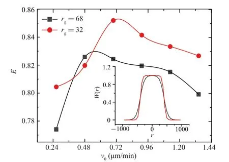
Fig.9.The relationship curve between the spatial search efficiency E with W(r)and the characteristic velocity v0 in P(v)of the cell colony.The inset is the corresponding spatial search weight W(r) curve.The black line and the red line correspond to rg=68 and rg=32 in Eq.(6),respectively.

In fact, we can always detect whichW(r) can make the maximum spatial search efficiencyEcorresponding to the velocity distributionP(v,v0= 0.72 µm/min) obtained through experiments by continuously changingW(r).In the simulation, we fixr0in Eq.(6) as the average width of spores,r0≈600µm, and continuously change the value ofrgto obtain different spatial search weight curvesW(r).As shown by the red line in Fig.9, when a suitable spatial search weight curveW(r)is found,the best search efficiency occurs atv0=0.72 µm/min (experimental result).In comparison to the red and black curves in Fig.9, a wider flat top of theW(r)curve corresponds to a largerv0in Eq.(2),as expected.From Fig.9,it can be seen that the velocity distributionP(v)of cells in experiments, modulated under a specific spatial search weightW(r), indeed corresponds to the optimal search efficiencyEof cell colonies.This means that the information of the spatial search weight of cell colonies is essentially contained in the velocity distribution of cell colonies.

8.Discussion

The spatial search weight should be the result of cell historical evolution[24]and related to the distribution characteristics of food in their growth environment.[23]In areas with scarce food, the distribution ofW(r) of cells maybe wide,and cells need to go far to find food.In areas with abundant food,the distribution ofW(r)of cells maybe narrow,and cells are more likely to search for food in the vicinity of spore areas.Since the cells in our laboratory have the same historical origin and the same real environment, they should have the same characteristics of spatial search weight distributionW(r).However, the spatial search weight distributionW(r)of the same cell colony may still change.For example, as the duration of cell planting time progresses,the spatial search weight distributionW(r)may change(if there is a change,it is reasonable).In our experiments,we have observed that the velocity distributionP(v)of cells will change significantly with the length of cell planted time.Whether this change is a direct reflection of the aging effect of spatial search weight distributionW(r) is a question that we want to explore further.The measured velocity distribution of cell colonies may still be different under different experimental conditions.For example,they can be influenced by factors such as the initial cell seeding density or the concentration of artificially added cAMP in the culture dish,as the collective behavioral characteristics of the resulting biological population are often closely related to the efficiency of interactions among organisms.[25]How to obtain reliable spatial search weight distributionW(r) from the optimum velocity distributionP(v) of cell colonies is still a challenge.

9.Summary

In this article, we seek to understand the speed distribution of cell movement in cell communities from the perspective of cell search efficiency.Based on the definition of cell search efficiency, the specific speed distribution of cell communities can correspond to the optimal spatial search efficiency of the cell community.Experimental findings suggest that the speed distribution of Dicty cells,under spatial search weight modulation,always corresponds to the optimal spatial search efficiency of the cell community.Our model explains the relationship between the distribution of cell spatial search weights and the speed distribution of cell movement, showing their intrinsic correlation.The deep information contained in the current speed distribution of cells is the spatial search weight distribution information during cell spatial search.In fact, we also provide a possible method to infer the spatial search weight based on the speed distribution of movement:by continuously adjusting the spatial search weight distribution under given speed conditions,we can calculate the change in search efficiency with the spatial search weight.Hence,the spatial search weight that corresponds to the optimal search efficiency represents the actual weight of cell movement during spatial search.Our work opens up directions for future research,where different conditions such as density and planting time can be studied to investigate whether the spatial weight of cell search movement obtained will also change.

Acknowledgement

Project supported by the National Natural Science Foundation of China(Grant No.31971183).