
Epidemic threshold influenced by non-pharmaceutical interventions in residential university environments
2024-02-29 09:20ZechaoLu卢泽超ShengmeiZhao赵生妹HuazhongShu束华中andLongYanGong巩龙延
Chinese Physics B 2024年2期
关键词:华中
Zechao Lu(卢泽超), Shengmei Zhao(赵生妹), Huazhong Shu(束华中), and Long-Yan Gong(巩龙延),†
1Institute of Signal Processing and Transmission,Nanjing University of Posts and Telecommunications,Nanjing 210003,China
2College of Science,Nanjing University of Posts and Telecommunications,Nanjing 210003,China
Keywords: epidemic threshold, susceptible–infected–recovered model, non-pharmaceutical interventions,time-varying heterogeneous contact networks
1.Introduction
In universities, the student population size is generally large, and students are in intimate contact, so infectious diseases spread more easily.Many research works have proposed models to study COVID-19 spread in such settings.[1–6]For instance,Hekmatiet al.studied the airborne transmission risk associated with holding in-person classes on university campuses.[1]Borowiaket al.used mathematical models to evaluate strategies that suppress the spread of the virus,specifically in dorms and in classrooms.[2]When there is an epidemic outbreak, non-pharmaceutical interventions (NPIs) are effective methods to contain infection and delay spread, and include isolation of ill individuals, quarantine of exposed individuals, face mask usage, nucleic acid testing, cancellation of mass gatherings, and school and workplace closures.[7–12]However,their real-world influence remains uncertain.[13]It is interesting to propose models to give quantitative evaluations in university environments.
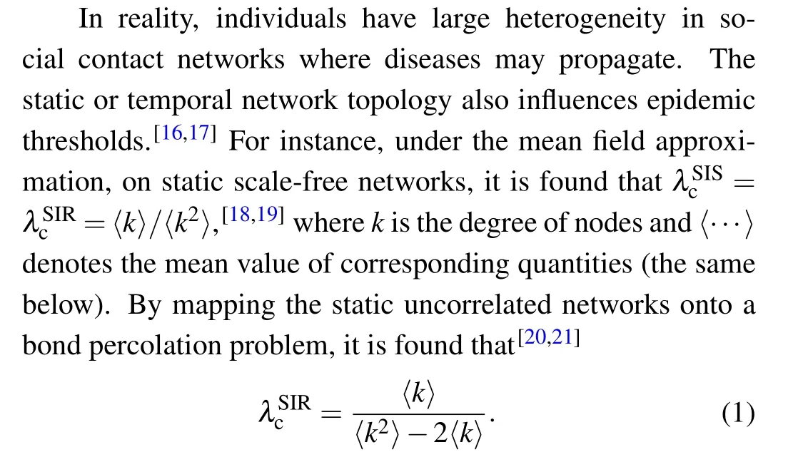
Epidemic threshold may be the important feature in the dynamics of an epidemic, which separates the healthy phase from the infected ones.To characterize it, mean-field compartmental models have been proposed and extensively studied,[14]where individuals belong to susceptible (S), infected (I), recovered (removed) (R), quarantine/isolation (Q),or other disease states (compartments).The population is supposed to be homogeneous mixing, and the evolutions of compartments are described by a group of non-linear differential coupling equations.For the SIR model,[15]the epidemic thresholdλc= 1, whereλ=β/µ.In Ref.[16],βandµare called transition rates for infection and recovery, andλis called the spreading rate or effective infection rate.
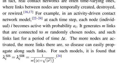
It is known that network structure and human mobility greatly influence the dynamics of an epidemic.[25,26]However,it is a challenge to create models that capture real-world dynamics in complex systems.[17]Traditional math models neglect the heterogeneity in social contact networks.[14,15]Static heterogeneous networks omit human mobility.[18–21]These time-varying heterogeneous contact networks are far away from the real world.[22–24]In recent years, agent based, spatially structured models have attracted a lot of attention,where the discrete nature of individuals, their mobility and stochastic contacts are considered.[6,7,16]Such models can capture the spreading patterns at the level of single individuals.Based on such models, disease spreads in social networks are studied, such as households, schools, workplaces and stores.[7,16]Compared with other social networks, in universities the student population size is generally large,and students regularly have classes, have meals and go to sleep, where they are in intimate contact.So the university environment is a paradigm of temporal contact networks.With Monte–Carlo simulation methods,we will study how disease propagates in universities using the full-scale stochastic agent-based model.[6]In close environments,maintaining physical distancing is an available NPI and is the most often used.We consider NPIs including using larger classrooms, adopting staggered dining hours and/or decreasing the number of students per dorm.The influences on the epidemic thresholds are explored.The underlying mechanisms will provide scientific evidence to control epidemics in universities.
The remainder of the paper is organized as follows.In Section 2 we introduce the model and related quantities.In Section 3,we present the numerical results.Finally,we summarize and conclude in Section 4.
2.Model depiction and related quantities
We simulate the epidemic spread in residential universities with a full-scale stochastic agent-based model.[6]Monte–Carlo simulation methods are used.In models, we trace the movements of all students, which include having classes in classrooms,eating at dinner halls and sleeping in dorms;they randomly choose seats in classes and to have meals.We record everyone’s health status,i.e.,S,IorR,as they attend activities.Every day, the simulation data of the numbers of infected individuals and recovered individuals are collected.Details are as follows.
2.1.Disease spreading process
We presume the SIR disease spreading process.[14,16]At every moment, each individual belongs to theS,IorRdisease state(compartment).For then-th individual, this is represented byXn,whereX=S,IorRandn=1,2,...,N.Suppose thatβandµare the transition rates for infection and recovery.[16]For a time interval ∆t,with transition probabilityβ∆t,a susceptible individual will change to an infected one if he is in contact with infected individuals.The largerβis,the more easily the disease spreads among people.At the same time,infected individuals will recover their health with transition probabilityµ∆t.And the recovered individuals will not be infected again.The variations of disease states can be written as
where them-th individual with stateIis the person in contact with then-th individual.In simulations,after ∆t,disease states for all people simultaneously update.
2.2.Time-varying and heterogeneous contact networks in residential universities
There are a large number of individuals, including students, faculty, and staff, in campuses.Due to a high studentfaculty ratio at universities, for simplicity we only consider the behaviors of students.[1]Each student is enrolled in a class.Students go to classes according to their class schedules.Schedules are regular for every week.For some courses,students may have joint classes.The members are fixed for each course.We suppose all students have their breakfast, lunch,and supper at dining halls,and at dining tables they may touch students of other classes.Each student is assigned a dorm,and the roommates are fixed.
Students mainly pack into classrooms, dining halls or dorms.Due to epidemic prevention, they are loosely connected in other zones.As pointed out in Ref.[27], on the weekends, the contact networks in universities are more loosely connected,with fewer users interacting with study participants.At the same time,school administrators advise students to maintain social distancing.So, for simplicity, during these times,except for bedtime in dorms,we omit disease spreading,but individuals can recover.If an individual enters a zone, the individual randomly selects a position and stays there until he/she leaves the zone.[6]Students move from one zone to another ones.For an individual, the people he/she is in contact with and the number of people will vary with time.In this sense, his/her contact networks are time-varying and heterogeneous.
2.3.Procedure of simulation
Suppose a residential university hasNcclasses.It has statistical data about the(frequency)distribution of weekly class hoursρwch, the distribution of class sizeρcsand the distribution of the number of joint classesρnjc.It also provides the school’s daily schedule.
Triple parameters (ηc,ηd,nd) are introduced, which are the seat occupancy rate in classrooms,the seat occupancy rate in dining halls and the number of students per dorm, respectively.They can be taken as averaged values of corresponding quantities.First,they relate to the degree of subnetworks.Second,they quantitatively characterize classroom capacity,staggered dining hours and dorm capacity, which relate to NPIs.So they are important parameters in our models.
Each classroom and each dining hall are simulated by square lattice networks.If an individual stays at lattice(i,j),the nearest and next nearest lattices (i±1,j), (i,j±1) or(i±1,j±1) may be occupied.He/she is in contact with the individuals who stay at these lattices, and the individuals at other lattices are omitted.Each dorm is simulated by a fully connected network,i.e.,an individual is in contact with all the other members of the dorm.
The procedure of stochastic simulation is as follows:
(i) The number of classesNcis set.Class sizes are randomly selected from the distribution of class sizeρcs.Each student is assigned a unique identifier numbern.
(ii)A class schedule is generated for each class.Weekly class hours are randomly selected from the distributionρwch.For each course, joint classes are randomly selected from the distributionρnjc.Based on the school’s daily schedule, the time for each course is randomly arranged.In a classroom,the number of seatsncseat=[ρcsρnjc/ηc],where[z]denotes the integer ofz.In dining halls,the number of seatsndseat=N/ηd.In classrooms and dining halls, students randomly choose seats.And there arendstudents in each dorm.
(iii) The recovery rateµand the effective transmission rateλare set.Then the infected rateβ=λµ.
(iv) Initially, one student is randomly selected from allNstudents and we set his/her disease state asIand all other students’states asS.
(v)From Monday to Sunday,based on the school’s daily schedule and the class schedules,an individual goes to dining halls,goes to classrooms if he/she has classes,stays at dorms,and so on.
If an individual stays in one zone for a time interval ∆t,a susceptible individual becomes infected at a rateβ∆tif he/she is in contact with infected individuals, an infected individual becomes a recovered one at a rateµ∆t, and a recovered individual stays recovered [see Eq.(2)].(Disease) states of all individuals are updated in parallel.
(vi)Repeat the(v)-th step until there are no infected individuals,then simulation for one cycle is completed.
(vii) Repeat steps (i)–(vi) to apply simulation for other cycles.
University environments are temporal contact networks,where the prevalence rate of COVID-19 depends on the infected rate, the recovery rate, the contact rate of individuals,and others.In the models, the infected rateβand the recovery rateµare independent variables.Recovery time from a disease depends on ages,overall health and other factors.For COVID-19, research suggests that it could take 2 weeks for someone to get over a mild illness or up to 6 weeks for severe or critical cases.[28]In our studies, to reduce the number of parameters, we fixµ=1/14 day-1and varyβ.At the same time,we define the effective infected rateλ ≡β/µ,[16]so it is a tunable parameter.The largerλis,the larger the probability an individual may be infected.
In simulations,everyone’s disease state evolves based on Eq.(2).The time interval ∆t=45 mins for each class,∆t=30 min for each meal, and ∆t=8 hours for sleep.In numerical simulations, we transfer all units to minutes.The system works day after day and week after week,until there are no infected individuals.At 22:30 every day,the data of the number of infected individuals and recovered individuals are collected,which will be used to characterize dynamic behaviors of systems.
2.4.Related quantities
For SIR models,NS(t)+NI(t)+NR(t) =N, whereNS(t),NI(t)andNR(t)are the number of individuals with stateS,IandR, respectively.Astincreases,NS(t) will decrease,NR(t) will increase, andNIfirst increases to a peak, then decreases to zero.[16]After enough time, there are no infected individuals.The final epidemic size is defined by
In fact,r∞can play the role of an order parameter to detect healthy-infected phase transitions.[16]In healthy phases,r∞are zeros,or are very small and can be ignored.In infected phases,r∞are finite values.
The fluctuations of final epidemic sizes are often large near the epidemic threshold.In order to identify the epidemic thresholds in finite system sizes,we also study the variability ofr∞,which is defined by[29–32]
Here〈z〉is the ensemble average ofz.In physics,it is a standard method to determine the critical point in the equilibrium phase of a magnetic system.[33]It may exhibit a peak atλp.For finite systems, it is used to approximate the epidemic thresholdλc.The validity of the numerical identification method has been confirmed for the SIR model in network models.[31]
The outbreak durationτis another basic quantity.[16]When a system approaches a critical transition or a tipping point, the system may return more slowly to its stable states under small perturbations,[34]i.e., the critical slowing down phenomenon.It can be used as early warning signals of infectious disease transitions.[35]We use the definition in Ref.[32],which is
where
3.Results
The reality of Nanjing University of Posts and Telecommunications (NJUPT) is used as an example.In Figs.1(a)–1(c), we plot the distribution of weekly class hoursρwch, the distribution of class sizeρcs, and the distribution of the number of joint classesρnjc,respectively.From Fig.1(b),we find that the mean number of students in each class is 31.9.

Fig.1.(a) The distribution of weekly class hours ρwch, (b) the distribution of class size ρcs,and(c)the distribution of the number of joint classes ρnjc,respectively.
From Monday to Friday, the school’s daily schedule is as follows: 7:00–7:30 breakfast;8:00–8:45,8:50–9:35,9:50–10:35,10:40–11:25 and 11:30–12:15 are the 1st to 5th classes,respectively; 12:30–13:00 lunch break; 13:45–14:30, 14:35–15:20,15:35–16:20 and 16:25–17:10 are the 6th to 9th classes,respectively;17:30–18:00 supper break;18:30–19:15,19:25–20:10 and 20:20–21:05 are the 10th to 12th classes; 22:30–6:30 sleeping.
3.1.No interventions
Based on the resources(the number of classrooms,dining rooms and dorms)of NJUPT and the total number of students in NJUPT,we set(ηc,ηd,nd)=(0.8,0.7,6),which is the baseline scenario,i.e.,the no interventions case.Results are shown in Fig.2.For eachλ, data for 100 cycles of stochastic simulations are given.More simulation cycles give similar results.The vertical blue lines are for the functionλ=0.52.
In detail, the final epidemic sizer∞versus the effective infected rateλis plotted in Fig.2(a).It shows that data almost overlap for the number of classesNc= 150, 300 and 600, which means such sizes can reflect statistical properties of systems.Whenλis relatively small,r∞is relatively small and approaches zero,which corresponds to the healthy phase.Whenλis relatively large, the values ofr∞are divided into two branches: in the bottom one,r∞is relatively small and approaches zero,[36]and in the top one,r∞is finite and increases withλ, which corresponds to the infected phase.In fact,r∞plays the role of order parameter to detect phase transitions.[16]The epidemic thresholdλcdetermined byr∞should be in the thermodynamic limit.[16]For finite systems, Fig.2(b) shows that the variability∆exhibits a peak atλ=0.52, which is used to approximateλc.[29–32]As there are two branches inr∞at relatively largeλ,in calculating∆,data forr∞>0.05,i.e.,the top branch ofr∞,are considered.Further,Fig.2(c)shows that the outbreak durationτis maximal nearλ=0.52,which also signals the epidemic threshold.
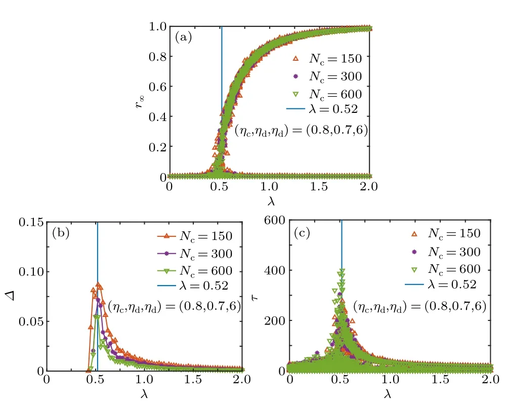
Fig.2.(a) The final epidemic size r∞, (b) the variability ∆and (c) the outbreak duration τ versus the effective infected rate λ at(ηc,ηd,nd)=(0.8,0.7,6),respectively.The number of classes Nc=150,300 and 600,respectively.The vertical blue lines are for the function λ =0.52.Data for 100 stochastic simulations are given.
3.2.Non-pharmaceutical interventions
We set (ηc,ηd,nd) equal to (0.8,0.3,6), (0.8,0.7,3),(0.4,0.7,6) and (0.4,0.3,3), respectively, which are labeled NPI-I,NPI-II,NPI-III and NPI-IV scenarios,respectively.At least one of their components is smaller than that for the baseline scenario[no interventions,(ηc,ηd,nd)=(0.8,0.7,6)].In practice,the methods of small class teaching(or being designated a larger classroom),staggered dining hours,and renting social housing can realize the required conditions.
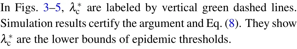
For the four NPI scenarios,we plot the final epidemic sizer∞versus the effective infected rateλin Fig.3.The number of classesNc=300 is used as an example.For each scenario,there exists an epidemic thresholdλcseparating the healthy phase from the infected phase, which is labeled by a vertical blue line.The correspondingλccan be numerically estimated from Figs.4 and 5, at which the variability∆and the outbreak durationτexhibit peak values.In calculating∆, data forr∞>0.05 are taken into consideration.
Eqnarray (1) gives the theoretical prediction ofλcfor static uncorrelated networks.[20,21]As the underlying networks we study are time-varying heterogeneous contact ones,inspired by Eq.(1)we define
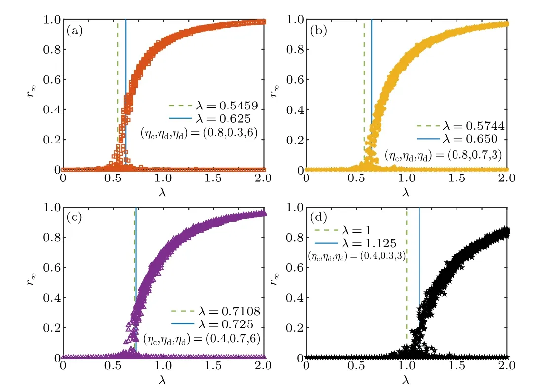
Fig.3.The final epidemic size r∞as a function of the effective infected rate λ for (ηc,ηd,nd) equal (a) (0.8,0.3,6), (b) (0.8,0.7,3), (c)(0.4,0.7,6) and (d) (0.4,0.3,3), respectively.The number of classes Nc =300.The vertical lines are for some values of λ.Data for 100 stochastic simulations are given.
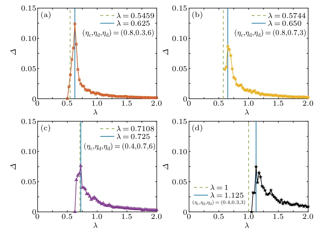
Fig.4.The same as Fig.3, but the variability ∆as a function of the effective infected rate λ.
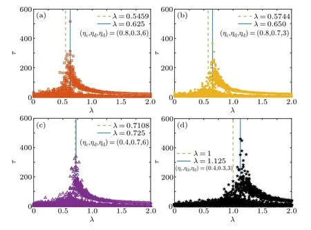
Fig.5.The same as Fig.3, but the outbreak duration τ as a function of the effective infected rate λ.
wherekis the degree of nodes and〈···〉tdenotes the time mean of the corresponding quantities.At the healthy-infected phase transition point,
In our model,students have much leisure time and during these times individuals can recover but not be infected.SoWis the ratio of the time spent having classes,having dinner and sleeping in dorms to all time.On the other hand,atβ/µ>1,i.e.,infected rateβis greater than recovery rateµ,due to the heterogeneity and randomness in social contact networks,a finite value ofr∞may occasionally occur.Combining the two aspects,the epidemic threshold can be approximately evaluated by
3.3.Comparing no interventions with non-pharmaceutical interventions
Table 1 gives the epidemic thresholdsλ*cobtained from Eq.(8)and the epidemic thresholdsλcnumerically estimated by the peaks of the variability∆(the outbreak durationτ).At the same time,to illustrate visually differences between them,we also plot the bar graph forλ*candλcin Fig.6.From them,we find NPIs can raise epidemic thresholds.In the NPI-III scenario,larger classrooms are used.Compared with the NPII and NPI-II scenarios,λ*c(λc)is relatively large in the NPI-III scenario,so its effect on containing infection is relatively obvious.The reason is that classrooms are the main places that students stay and contagious disease spreads.Combination of interventions is the NPI-IV scenario and the corresponding effect is most significant.

Table 1.Table outlining the values of λ*c and λc.
For all scenarios, including no interventions and NPIs,the final epidemic sizesr∞are plotted together in Fig.7(a).The mean〈r∞〉 are also shown in Fig.7(b), where data forr∞>0.05 are taken into consideration.To give quantitative comparisons,we define the ratio
We plot the corresponding ratioKin Fig.7(c).This shows that at relatively smallλ,the effect of countermeasures is more obvious.All NPIs can reduce the outbreak size.For the combination of interventions,i.e.,(ηc,ηd,nd)=(0.4,0.3,3),K=7.8%atλ=1 andK=84.9%atλ=2,which has the most significant effect in reducing the outbreak size.
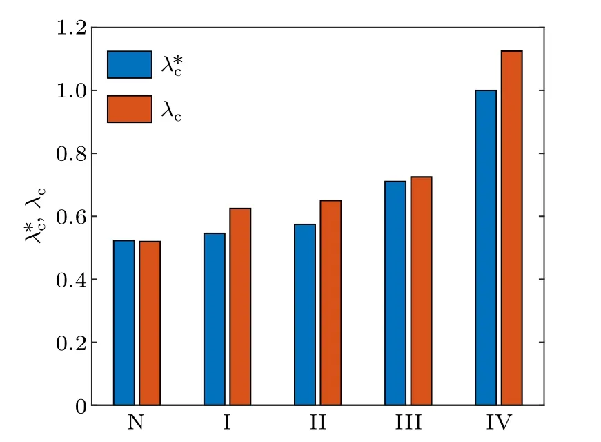
Fig.6.The bar graph for λ*c and λc, where N denotes the baseline scenario,and I–IV denote the NPI-I–IV scenarios.
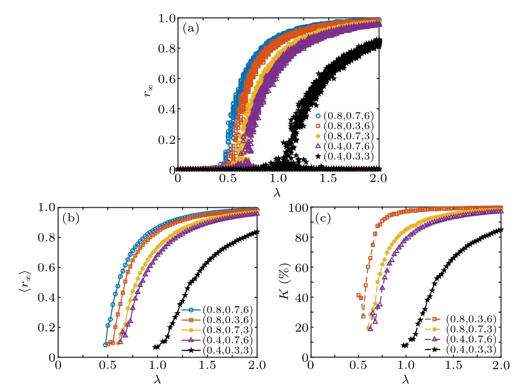
Fig.7.(a) The final epidemic size r∞, (b) the mean 〈r∞〉, and (c)the ratio K versus the effective infected rate λ, respectively, where(ηc,ηd,nd)equals(0.8,0.7,6),(0.8,0.3,6),(0.8,0.7,3),(0.4,0.7,6)and(0.4,0.3,3).The number of classes Nc =300.Data for 100 stochastic simulations are given.
4.Conclusion
The university is a typical social community.To quantitatively evaluate the effect of NPIs on containing infection,an agent-based SIR model with time-varying heterogeneous contact networks is proposed.The seat occupancy rate in classrooms,the seat occupancy rate in dining halls and the number of students per dorm are important parameters to characterize NPIs.We obtain epidemic thresholds for scenarios including no interventions and four kinds of NPIs.We make quantitative comparisons.We find the NPI of using larger classrooms plays an important role in raising the epidemic threshold and reducing the outbreak size.In fact, it can also be realized by reducing the number of students in a classroom,i.e.,dividing a class into several small classes.The effect of combination of interventions is most significant.All these studies provide scientific evidence to support the use of NPIs in campuses.
Acknowledgment
Project supported by the National Natural Science Foundation of China(Grant No.61871234).
猜你喜欢
凤凰动漫(军事大王)(2022年1期)2022-04-19
华中建筑(2021年12期)2022-01-17
湘潮(上半月)(2021年10期)2021-12-02
Chinese Physics B(2021年3期)2021-03-19
当代水产(2020年10期)2020-03-17
当代水产(2019年2期)2019-05-16
当代水产(2019年1期)2019-05-16
制造技术与机床(2018年12期)2018-12-23
制造技术与机床(2018年9期)2018-09-19
华中学术(2017年1期)2018-01-03

- Chinese Physics B的其它文章
- Unconventional photon blockade in the two-photon Jaynes–Cummings model with two-frequency cavity drivings and atom driving
- Effective dynamics for a spin-1/2 particle constrained to a curved layer with inhomogeneous thickness
- Genuine entanglement under squeezed generalized amplitude damping channels with memory
- Quantum algorithm for minimum dominating set problem with circuit design
- Protected simultaneous quantum remote state preparation scheme by weak and reversal measurements in noisy environments
- Gray code based gradient-free optimization algorithm for parameterized quantum circuit