Magnetic field regression using artificial neural networks for cold atom experiments

Ziting Chen(陈子霆), Kin To Wong(黃建陶), Bojeong Seo, Mingchen Huang(黄明琛), Mithilesh K.Parit,Yifei He(何逸飞), Haoting Zhen(甄浩廷), Jensen Li, and Gyu-Boong Jo

Department of Physics,The Hong Kong University of Science and Technology,Kowloon 999077,China

Keywords: ultracold gases,trapped gases,measurement methods and instrumentation

1.Introduction

Precisely calibrating the magnetic field inside a vacuum chamber is of experimental significance to various fields.For instance,a magnetic field is one of the common control knobs in the ultracold atoms experiment,enabling various studies on many-body physics[1]including Bose–Einstein condensation-Bardeen–Copper–Schrieffer (BEC-BCS) crossover,[2]formation of matter-wave soliton,[3–5]and Efimov states[6]through the Feshbach resonance that tunes inter-atomic interactions.[7]However, the demanding precision of the magnetic field imposed by these experimental controls and the inaccessibility to the vacuum chamber make calibration of the magnetic field a difficult and time-consuming task.Moreover,spectroscopic measurement,a typical approach to magnetic field calibration,is mainly sensitive only to the magnitude of the magnetic field.The magnetic field direction and its precise calibration are of critical importance for magnetic atoms (e.g., erbium or dysprosium)where the orientation of the magnetic dipole moment plays a critical role.[8,9]

Recent years have witnessed the great success of neural network (NN) applied to assist experiments, including multiparameter optimization of magneto-optical trap,[10,11]optimization of production of Bose–Einstein condensate,[12–15]and recognition of hidden phase from experimental data.[16–19]In this work, we introduce a novel method to precisely determine the magnetic field vectorB= (Bx,By,Bz) inside a vacuum chamber with the assistance of an NN.Since the target position inside the vacuum chamber is typically inaccessible,we detect magnetic fields at several surrounding positions,which are sent to the trained NN that is able to accurately deduce the magnetic field inside the vacuum chamber.We apply this method to our apparatus of erbium quantum gas,[20–22]which has a large magnetic dipole moment making it particularly sensitive to magnetic field vector.[23,24]We present the details of the NN-based method,including setting up the simulation model,training process,and final performance.For simplicity, magnetic field data for training and validation of NN is generated by a standard finite-element simulation package from COMSOL Multiphysics electromagnetic module,[25]instead of experimental measurement.Moreover,we systematically investigate the impact of the number of three-axis sensors at surrounding positions and the magnitude of the magnetic field on the performance of the method providing a practical guide for implementation.In contrast to previous works,[26–30]which predict the magnetic field vector across a wide experimental region,our goal in this work is to extrapolate the magnetic field vector at a specific position within an inaccessible region.Our approach provides a simple method for monitoring magnetic fields without requiring any prior knowledge of the solution of the Maxwell equation.

2.Methodology

The implemented machine learning algorithm is an artificial NN.A typical NN is formed by multiple layers of neurons where each neuron stores one number.The first and last layers of the NN are the input and the output layers respectively while all the layers between are hidden layers.Neurons between adjacent layers are connected with varying weights where the neuron values are determined by those in the previous layer through the calculationy=σ(∑i wixi+b),whereyis the neuron’s value andbis the bias of the neuron.wirepresents the connection weight between the neuron and one neuron in the previous layer wherexiis the corresponding value of that neuron.It is important to notice if the calculation only usesxiandb, the NN will ultimately be reduced to be a linear function only.To introduce nonlinearity into the NN, the values are passed through an activation functionσ.A common and useful activation function is the rectificed linear function(ReLU),which is defined to be ReLU(x)=max(0,x).The complexity of the NN is determined by the layers and neurons since they increase the number of calculation done within the NN.In general,there is no restriction on the number of layers and number of neurons in each layer.They can be tuned freely based on the complexity of the problem.

To obtain the right output from the NN,the neurons’parameters(weight and bias)are tuned through training.During training,a loss is calculated based on the output of the NN and the correct output.The loss is then minimized through an algorithm called optimizer.Many optimizers including the Adam optimizer are just variations of the gradient descent algorithm.The gradient descent algorithm calculates the gradient of the loss with respect to the neurons’parameters.Then,the parameters are tuned in the same direction as the gradient such that the reduction in the loss is maximised.After a certain number of training iterations, it is possible that the NN will be overtrained if more iterations are run.Overtraining the NN causes it to produce more accurate results for the training data but decreases the NN’s accuracy for other data.To prevent overtraining, the loss of another separate data set (validation data set)is used to keep track the NN’s performance on other data sets.Based on the problem that needs to be solved, we may want to evaluate the performance of the NN using loss functions that differ from the one used in training.In that case,another data set is needed.

Characterizing, training and testing the NN are coded by using common Python packages like Tensorflow and Pytorch.[31,32]These packages have many common and complex algorithms prewritten in them so that we only need to specify several parameters to run the machine learning algorithm.

The magnetic field measured by three-axis sensors outside a vacuum chamber is fed into the NN,which predicts the magnetic field at the center of the chamber.Hence, the function of the NN is to act as a hyperplane that relates the magnetic field at different spatial points.Regressing such a hyperplane would require a substantial amount of data.Obtaining training data from a real experimental setup,though it can take into account every factor,is difficult and time-consuming.Instead,we generate training data from finite element simulation using COMSOL Multiphysics.As long as the simulation model takes into account important factors, simulation data would be a reliable substitute for real data.

The simulation model is shown in Fig.1,which contains a science chamber commonly used in cold atoms experiments.Originally,the chamber is made of materials including 314L,304 stainless steel,aluminum,glass,and plastic.However,to reduce computational time, non-magnetic parts of the chamber are removed as they do not affect the result,and only parts made of 314L and 304 stainless steel are kept.314L and 304 stainless steel, under low strain and irradiation, can be considered as linear materials with no hysteresis loop.[33]In addition, only a static magnetic field is of concern for most experiments.Therefore, we only need to simulate the magnetic field under time-independent conditions.In order to generate a stable magnetic field,three pairs of copper coils with constant current are placed around the chamber along three orthogonal directions, mimicking the coils used in experiments.To account for the Earth magnetic fieldBEarthin the laboratory, a constant 400 mG magnetic field is added in thex-direction.To notice,when adopting this method,it is important to check the direction and magnitude ofBEarthbefore training the NN since they can vary in different locations.

Even though simulation data is much easier to obtain than real data,simulation of each datum still requires a significant amount of time.To diminish data acquisition time,we exploit the linearity of Maxwell’s equations that any superposition of solutions is also a valid solution for linear materials.By virtue of this,the whole output space can be mapped using only three linear independent results,which can be obtained by simulating each pair of coils in the model.Using these results, we obtain new data that is not redundant and form a large data set.

As shown in Fig.2,after setting up the simulation model and obtaining the simulation data, we input the data into the artificial NN for training and prediction testing.The implemented NN contains two fully-connected hidden layers with ReLU as activation functions.During the training, the neurons’ parameters of the NNs are adjusted to minimize the root-mean-square error (RMSE) loss function using the Adam optimizer.[18]This is a common loss function for regression and can be defined as RMSE =wherenis the number of data,Bactualis the actual output,Bpredictis the predicted output by NN andαdenotes the component of the magnetic field along three spatial dimensions.The total number of simulation data is 1.5×105,80%of which is used for training while 20%is reserved for validation.When the validation loss isn’t improving for several epochs,the training is terminated to prevent overtraining.However, it should be noted that RMSE could not reflect the statistic of the error for each measurement.

To properly evaluate the performance of the NN-based magnetic field regression,we define a relative prediction error(RPE), which is the vector difference between the actual and predicted output divided by the magnitude of the actual output

This value is evaluated from another data set of size of 105.We calculate the RPE from each datum to form a set of errors and extract the upper bound of the RPE,below which 90%of data points would be accurately estimated.

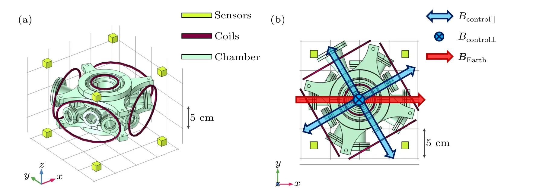
Fig.1.Schematic of the simulation model.(a)Overview of the model.The main body of the model is an experimental chamber in an ultra-high vacuum environment.The control magnetic field Bcontrol is generated by three orthogonal pairs of copper coils.Several three-axis magnetic field sensors surrounding the vacuum chamber are indicated in light yellow.(b)Top view of the model.Exemplary magnetic fields(blue arrows)generated by coils are shown.A red arrow is also added to show the Earth’s magnetic field in the model which is set to the x direction.

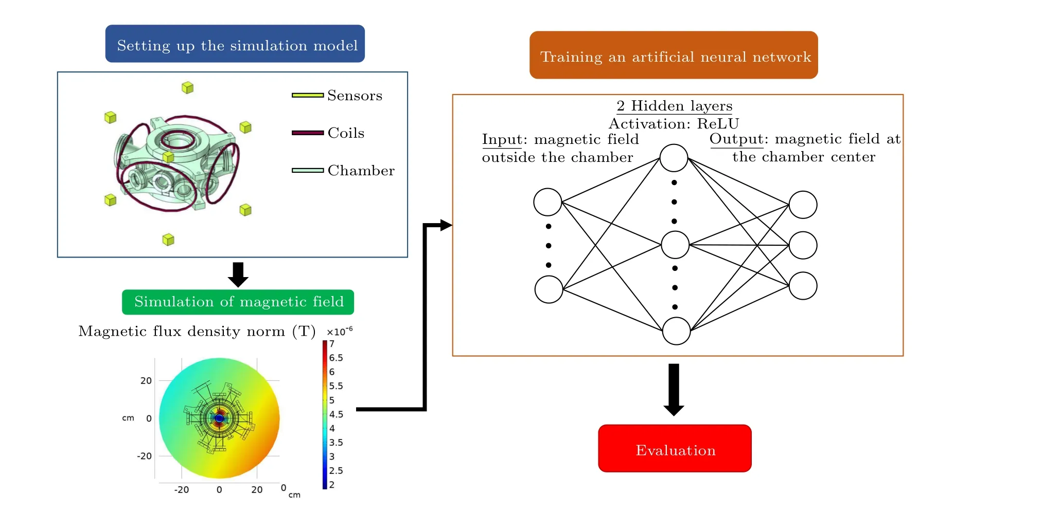
Fig.2.Training an artificial neural network.First,a simulation model which contains a science chamber and coils as magnetic field sources is set up.Then,the model is simulated to obtain data that is passed into an artificial NN for training.The NN has four layers: the input layer which is the magnetic field measured by sensors outside the chamber,two fully connected hidden layers with ReLU as activation functions,output layer which is the target magnetic field at the chamber center.At last,the prediction of the NN is evaluated.

3.Interpretation of the training process

To fully evaluate the NN’s performance,it is essential to first grasp the purpose of training the NN or specifically, the target equation of the regression.In theory, the hyperplane relating magnetic field at different spatial points can be calculated using Maxwell’s equations directly.By substituting the spatial coordinates of the target point into the general solution, we remove its spatial degree of freedom, causing the output to depend only on the integration constants that are determined by the boundary conditions.However,the boundary conditions can just be the magnetic field at other spatial points.Hence,in principle,we can extract a hyperplane from the solution that serves the same function as the NN.Since this hyperplane is entirely based on Maxwell’s equations, its output must always be correct.Therefore,the goal of training the NN is to reduce the gap between the NN and this ideal hyperplane.

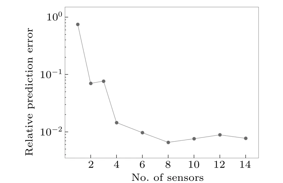
Fig.3.Relative prediction error of magnetic field RPE of the magnetic field at the center of vacuum chamber predicted by NN using varying numbers of sensors.The vertical axis is in logarithmic scale.The RPE plummets when the number of sensors increases from 1 to 6.Afterward, the RPE stays in the same order of magnitude and varies nonsystematically.

To have a better understanding of the relation between Maxwell’s equations and the NNs, we look at how the RPE depends on the number of sensors.As shown in Fig.3, the RPE drastically reduces when the number of sensors increases to 6 and has a similar value onward.This dramatic reduction can be explained by the number of boundary conditions required to identify the hyperplane from directly calculating Maxwell’s equations.The required number of boundary conditions for the unique solution of the Maxwell’s equation,equals the product of the number of independent variables,the order of differential equation,and the number of components of the magnetic field.For a time-independent Maxwell’s equation,the required number of boundary conditions is 18(3×2×3).Since the boundary conditions are provided by magnetic field measured at different spatial positions by sensors, to obtain a unique and accurate result,6 sensors are required minimally,where each three-axis sensor measures 3 components of the magnetic field.This,together with the claim that the NN is approximating the ideal hyperplane calculated from Maxwell’s equations,explains the rapid reduction of RPE in Fig.3.When below 6 sensors are used, the NN does not have enough information for the ideal hyperplane to calculate the unique result.Therefore,the trend in Fig.3 indicates a strong relation between the NN and Maxwell’s equations,strengthening the claim that training the NN is equivalent to bringing the NN closer to the ideal hyperplane calculated from Maxwell’s equations.Our observation is consistent with another early work,[30]which demonstrated that the solution of the Maxwell’s equation can be approximated by the NN trained with sufficient amount of data around the target point.On the other hand, however, it is crucial to notice the NN can only approximate the ideal hyperplane but never reach it since their mathematical forms are fundamentally different.Hence,errors always exist from the network’s prediction.Besides, the quality of the approximation greatly depends on and is limited by the training conditions and data.This aspect of the network will be clearly shown in the following result.

4.NN’s performance over a range of magnetic field

In this study, we evaluate the performance of the neural network under various magnetic fields created by the coilsBcontrol,ranging from 0.6 G to 100 G.These values cover the typical range of magnetic fields used in experiments involving ultracold dipolar atoms.[21]This can be achieved by generating multiple prediction data sets with different average magnitudes of output.Before commencing the test,it is crucial to consider the average magnitude of the output of the training data since it could significantly affect the training process that determines the network’s response to different magnetic fields.

Figure 4(a)illustrates the accuracy of the NN in predicting the magnetic field at the center of the chamber under different magnetic field conditions.When the NN is trained with weak magnetic field strength(Bcontrol)of 1 G–5 G,the error is minimized within this range and can be reduced to as low as approximately 0.2%.However,when the NN is trained with a strong magnetic field strength of 10 G–50 G,the error is minimized between 30 G to 50 G.Additionally,when theBcontrolis outside of the specified range, the error rapidly surges to above 10%.This issue could be avoided if the magnetic field was completely rescalable.Unfortunately,due to the presence of the constant Earth magnetic fieldBEarth,this is not possible.AsBcontrolchanges, so doesBEarth/Bcontrol, and these variations can be drastic, particularly whenBcontrolchanges by an entire order of magnitude.If the NN is trained with a weak magnetic field strength,there is a possibility that the network would calculate the bias based onBEarth/Bcontrolfor a weaker field even whenBcontrolis much stronger, leading to a higher error.This also explains why the applicable range ofBcontrolfor NN trained at weakerBcontrolis narrower,asBEarth/Bcontrolvaries much faster at weaker magnetic field strengths.

To expand the applicable range of the NN,one option is to train it on a larger range ofBcontrol.However, this method has been proven to be ineffective, as shown in Fig.4(a).The figure demonstrates that the errors are very similar between the NN trained with both weak and strong fields and the one trained with only strong fieldBcontrol, indicating that the neural network simply ignores weakerBcontrol.This is because the RMSE loss function is used in absolute value.LargerBcontrolusually produces larger absolute RPE, causing the network’s parameters to be tuned in a way that provides more accurate results at largerBcontrolover weaker ones.

Two viable ways to improve the working range of the NN are suggested here.First,the NN can simply be trained withoutBEarthin the data by adjusting the sensor offsets until the reading is zero or compensatingBEarthin the laboratory.Both of the methods involve removing the effect of theBEarthduring the training process.In Fig.4(b),the RPE of the network’s prediction can then be kept below 0.4%over the entire range when there is noBEarth.Therefore,this method is very effective in principle but requires good control over the sensors.

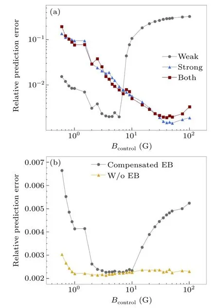
Fig.4.Relative prediction error under different training conditions RPE versus the magnetic field generated by the coils Bcontrol, covering from 0.6 G to 100 G.(a)The Earth’s magnetic field BEarth is present and compensated (assumed to be 400 mG).The legend shows in which range of field the artificial NN is trained.Weak refers to a field from 1 G to 5 G and strong refers to 10 to 50 G range.The error is minimized and reduced to around 0.2%over a range where the training field has a similar magnitude as the testing field.However,the error increases rapidly to over 10%outside the working range.The working range of the NN trained with a stronger field is wider (in log scale) than the one trained with a weak field.When the NN is trained with both weak and strong fields,the result is similar to the one produced by an NN trained with a strong field only.(b)BEarth (EB in the figure)is either compensated or removed entirely as indicated by the legend.For the one with compensated BEarth, the NN is trained with a weak field.The minimized region still remains but the increase in error is way less drastic outside the range compared to having full BEarth.The error can be suppressed under 0.7%over the whole range.For the one without BEarth, the NN is trained at 2.5 G.The performance of the network is very consistent over the whole range with errors around or below 0.3%.

The second method is to compensateBEarthusing coils in the laboratory to attenuate the effect ofBEarth.Although it is difficult to completely eliminateBEarth, it is possible to compensate for 90%in the laboratory.Therefore,we evaluate the effectiveness of this method by training NN with a small bias of 40 mG, which is displayed in Fig.4(b).The RPE is below 0.7%over the whole range and below 0.3%from 20 G to 100 G, indicating that excellent precision and wide working range can be achieved simultaneously with this method.

Nonetheless, even when both of the above methods are not applicable, the NN is still useful and powerful.As long as the approximate value of the magnetic field is known, the properly trained NN can always be picked to calculate the magnetic field with an extremely low error.When the order of the magnetic field is unknown, however, we can still use the NN trained with the wrong range to determine the order of magnitude, since the error is still over an order larger in this case.The more accurate result can then be calculated using the properly trained NN.

5.Application to cold atoms experiments

The performance of magnetic field regression demonstrated in this work opens a new possibility of applying this method to cold atoms experiments.One such system is an apparatus of dipolar erbium atoms which have a large magnetic moment of 7µBwhereµBis the Bohr magneton and contains a dense spectrum of Feshbach resonances.[24]Even at a low magnetic field regime, erbium atoms have multiple Feshbach resonances for a magnetic field smaller than 3 G, where the widths of these resonances are around 10 mG–200 mG.[23]The regression method could allow us to monitor the magnetic field vector with the resolution of∼10 mG over the range of 3 G,which is accurate enough to properly calibrate the experimental system.This is still favorable for other atomic species,such as alkali atoms, since a maximal RPE of the magnetic field is about 1.25 G in the range of 500 G, which is sensitive enough compared to the linewidth of most commonly used Feshbach resonances.[7]However, even though the regression method can provide useful results, we suggest that its accuracy should be verified with another method, such as radio-frequency spectroscopy.

Apart from precisely determining the magnetic field inside a vacuum chamber,the proposed method also serves as a quick indicator for magnetic field change.For instance,when sensors around the vacuum chamber give unexpected values,it indicates a change of magnetic field inside a vacuum chamber.If all 6 sensors are changed along the same direction,then an external magnetic field is suddenly introduced to the system.On the other hand,if these 6 sensors change in a different direction, then it is likely because the position of an electronic device within the area is changed.The former can be solved by compensating the external magnetic field by coils,while the latter requires to re-train the NN.The change of sensor value signals a change in the environmental magnetic field, which provides important information and is easy to monitor.

6.Conclusion

A simple method based on NN to extrapolate the magnetic field vector at a specific position within an inaccessible region is demonstrated.An artificial NN is trained such that it predicts the magnetic field at the center of the vacuum chamber based on the magnetic fields surrounding the chamber.The performance of trained NN is evaluated and the training process including the number of required sensors and training magnetic field magnitude is investigated.

After training, the RPE of magnetic field magnitude below 0.3% is achieved under a wide range of magnetic fields,which is sufficient to calibrate the magnetic field inside the chamber in our erbium quantum gas apparatus, where many narrow Feshbach resonances exist even in the low field regime.Besides, experiments with other atomic species can benefit from this method,not only in precisely determining magnetic field, but also serving as a robust monitor for environmental magnetic field.Furthermore, as no special setup is required,the established method can be extended to other magnetic field-sensitive experiments conducted in an isolated environment.

Acknowledgments

Project supported by the RGC of China (Grant Nos.16306119, 16302420, 16302821, 16306321, 16306922,C6009-20G,N-HKUST636-22,and RFS2122-6S04).