Numerical simulation of hemodynamic interactions of red blood cells in microcapillary flow*

SHI Xing (石兴), ZHANG Shuai (张帅), WANG Shuang-lian (王双连)

School of Aeronautics and Aerospace, Zhejiang University, Hangzhou 310027, China, E-mail: shix@zju.edu.cn

Numerical simulation of hemodynamic interactions of red blood cells in microcapillary flow*

SHI Xing (石兴), ZHANG Shuai (张帅), WANG Shuang-lian (王双连)

School of Aeronautics and Aerospace, Zhejiang University, Hangzhou 310027, China, E-mail: shix@zju.edu.cn

(Received July 18, 2012, Revised September 11, 2013)

The hemodynamic interactions of red blood cells (RBCs) in a microcapillary flow are investigated in this paper. This kind of interaction is considered as the non-contact mutual interaction of cells, which is important in the suspension flow of blood, but not sufficiently understood. The distributed Lagrange multiplier/fictitious domain method in the lattice Boltzmann framework is used to solve the suspension of the RBCs. The modification of the flow due to the cells, the dependence of the cell deformation on the flow and the cell-cell interaction via the fluid are discussed. It is revealed that the long-range hydrodynamic interaction with a long interacting distance, more than about 5 times of the RBC equivalent radius, mainly has effect on the rheology properties of the suspension, such as the mean velocity, and the short-range interaction is sensitive to the shape of the cell in the microcapillary flow. The flow velocity around the cell plays a key role in the cell deformation. In the current configuration of the flow and cells, the cells repel each other along the capillary.

erythrocyte, hydrodynamic interactions, fictitious domain method, lattice Boltzmann method (LBM), fluid-structure interactions

Introduction

The red blood cell (RBC) plays an important role in the oxygen delivery in the blood circulation. In the capillary, the behavior of the RBC determines the efficiency of the gas exchange between the RBCs and the tissues. If a multiple cell system is considered, the cell-cell interactions cannot be ignored. Generally, there are two kinds of cell-cell interactions, one is due to the interactions of the molecules to the RBC membrane[1,2]which will vanish quickly as the distance between the interactive surfaces increases, the other is the hydrodynamic interaction where the RBCs affect each other via the suspending fluid. For the first kind of interactions among the membrane molecules, some analytical or empirical equations were obtained from the experiments and theoretical models[1,2]. On the other hand, the hydrodynamic interaction is difficult to be predicted because it is determined by many mutually affecting factors, such as the flow conditions, the RBC shapes, the relative locations of cells and so on.

With the development of the computational capacity, the numerical simulations of the RBCs have been attracting an increasing attention. The simulations of an individual RBC provide a down-to-cell approach to study the blood flow. The behavior of a single cell in some typical flow is carefully studied. In shear flow[3-5], there are three kinds of motions of the RBC, the tumbling, the breathing and the tank trending, due to the differences of the flow and the cell properties. The controlling parameters are the Ca number defined as the ratio of the viscous force of the fluid to the membrane force, the membrane bending module and the ratio of the viscosities of the suspending fluids and the cytoplasm. With respect to the flow in a pipe[6], the studies are focused on the deformation, the migration, the distribution of the RBCs and the modification of the flow. But the direct simulation of the system with massive cells is still costy and unpractical. In themost recent simulation, the number of the involved RBCs in a 3-D simulation is about 2000[7]. Due to an acceptable cost and the importance in the blood circulation, the simulation of a few cells in the capillary is a natural starting step for the full simulation of the blood system.

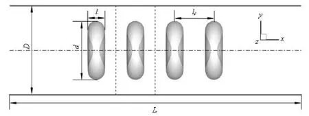
Fig.1 Schematic diagram of the problem setup

In the numerical simulation of a multi-cell system, the fluid-structure interaction with the moving fluid-solid interface is involved, where the complicated shape and topology are usually encountered. For the classical body-fitted algorithm, such as Arbitrary Lagrangian-Eulerian (ALE) method[8], the computational cost of the re-meshing procedure is high and one always fails in dealing with the large deformation and the complicated topology of the interface. So another series of algorithms, such as the boundary integration method[9], the immersed boundary method[10], the immersed finite element method[11], the fictitious domain method[12], were designed to overcome the difficulties. In these algorithms, the re-meshing is not necessary and it is convenient to adjust the large deformation of the fluid-solid interface. With the help of the proposed algorithms, the simulations of a multicell system were carried out. A lot of computations were performed based on the two dimension assumption[13,14]. Comparing to the 2-D simulations, the full three dimension simulations are still rare. Pozrikidis[9]analyzed a single file of the RBCs through the capillary by the boundary integration method. Zhao et al.[15]simulated several RBCs in a micro tube by the spectral boundary integral method. Liu and Liu[11]captured the rheology properties and the aggregations of the RBCs. However, the previous studies mainly focused on the rheology properties modified by the introduction of the cells and the deformation of the cells. In fact, for a low or moderate volume fraction blood flow, the cells are not close enough so that the adhesive force is not dominated and they are far enough to each other, where the interaction can be ignored, but the hydrodynamic interactions are important.

In this paper, the previously developed LBMDLM/FD method[16]is used to study the RBCs’ interactions via the fluid in a microcapillary. The LBMDLM/FD method is designed as a fixed mesh algorithm to avoid the remeshing procedure, which makes it suitable for the fluid-structures with large deformations. The flow is solved by the LBM and the coupling of the fluid-structure interaction is described by the distributed Lagrange method, one of the fictitious domain method. We will present the features of the flow, the deformation, the distribution of the RBCs and the hydrodynamic influence of the RBCs under some relatively simple flow and cell configurations.

1. Flow configuration and numerical descriptions

1.1 Problem setup and parameter definitions

The undeformed shape of the RBC is biconcave with an equivalent radius a, derived from a=(3V/ 4π）1/3, where V is the volume of the cell. From the experimental data[17], V=93 μm3, the equivalent radius is 2.82 μm. The schematic diagram of the flow and cell configurations is shown in Fig.1. The length of the capillary tube is L. In the present paper, the diameter of the capillary is fixed to D=3.3a. For convenience, the tube axis is parallel to the X axis and the flow direction points to +X. The cross section of the tube is parallel to the Y-Z plane. The RBCs are aligned to a single-file at a distance lcbetween two neighboring cells and with their centroids on the tube axis. The periodic flow conditions are applied on the inlet and the outlet of the tube. On the wall of the tube, no-slip condition is imposed. The viscosity of the cytoplasm is equal to that of the suspending fluid. The flow is driven by a body force, dp/dL, from a static state.

Several dimensionless parameters are used. The centerline velocity of the undisturbed parabolic flow is Umax. The characteristic time scale is defined as D/ Umax. The previous studies[4]show that the major dimensionless number, Ca, is the control parameter of the cell deformation, which is the ratio of the viscousforce of the fluid to the elastic force of the membrane, defined as

where Ucis the velocity of the cell,fμ is the fluid viscosity, andsμ is the membrane shear modulus. The deformation of the RBCs in response to an external force is usually measured by the deformation index (DI), defined as[18]

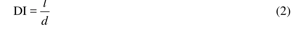
As shown in Fig.1, l and d are the length and the diameter of an RBC, respectively.

1.2 Red blood cell model

In the numerical simulation, the RBC can be modeled as a soft deformable particle or a Newtonian cytoplasm enclosed by the membrane made of the phospholipid bilayer supported by the protein skeleton. The latter one is more real to the micro bio-structure of the RBC. There are two kinds of membrane models at present. The macroscopic model is developed from the classic continuous elastic theory and is focused on the elastic properties, disregarding the details of the membrane structure. The other is a microscopic model, where the membrane surface is triangulated to represent the protein skeleton. In order to reduce the computational cost, a coarse-grained model of the RBC membrane was proposed[19,20]. In this paper, the Fedosov’s model[20]is adopted. The total energy of the system with the phospholipid bilayer and the skeleton is expressed as

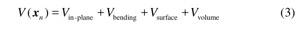
where xnrepresents the vertex coordinates and the inplane energy is combined with a wormlike chain with the energy Vwlcand a repulsive potential with the energy Vp

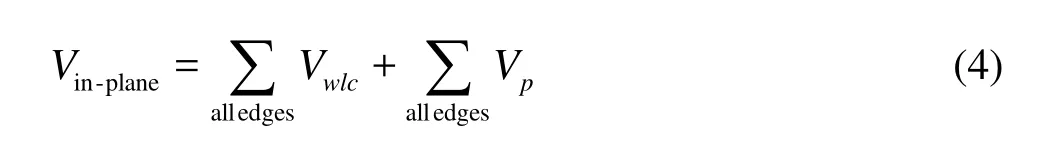
The details of the potential of the in-plane energy, the bending energy Vbending, the energy to constrain the surface Vsurfaceand the volume Vvolumecan be found in previous papers[19,20], The nodal membrane forces,, are derived from the total energy as follows

1.3 LBM-DLM/FD method

The distributed Lagrange multiplier method/fictitious domain method for an elastic body was proposed by Baaijens[12]and Yu[21]. If we use the LBM[22]in the flow solver and introduce the Lagrange multiplier, as a type of pseudo body force and as the external force term to the lattice Boltzmann equations, the LBMDLM/FD method can be constructed[16]. The full equations in the LBM-DLM/FD method are expressed as follows:

where fiis the single-particle distribution function in the i-direction of the microscopic velocity eiwith the corresponding equilibrium function, τ is the relaxation time,tδ denotes the time step, csrepresents the speed of sound. The weight factors wiare selected according to the LBM model. u is the velocity, ρ is the mass density, f is the body force, and σ is the stress. The subscripts f and s correspond to the fluid and structure variables, respectively. λ is the Lagrange multiplier.sφ and γ are the corresponding weighting functions. The RBC deformation in flow can be assumed to be in a quasi-equilibrium, and Eq.(7) is simplified in the form without the acceleration term as follows

where the force term is the sum of the body, membrane, fluid, and pseudo-body forces in the form of the Lagrange multiplier. The whole system is decoupled to the fluid and solid sub-problems by the fractional step scheme similar to the DLM/FD method[21].

2. Results and discussions

2.1 Grid convergence test and validation

In this test, the cells are distributed periodically along the tube. The distance lc=2.5a. The Capillary number and the Reynolds number based on Umaxare kept as 0.69 and 0.72, respectively. The mesh comparison involves both the solid mesh and the fluid grid. Three characteristic physical parameters are chosen for comparison and the results are shown in Table 1, where Ncis the number of nodes on the RBC membrane and NDis the number of the lattice along the tube diameter and Umax fis the maximum axial flow velocity in the tube. It is found that the mesh configuration with Nc=500 and ND=58 has a good enough resolution for the problem. In the test computation, another source is also found, resulting in a difference between the coarse and fine meshes, which is the resolution of the gap between the cell and the wall, where more than 4 grids are placed. The mesh configuration in the current paper is Nc=3 000 and ND=68.

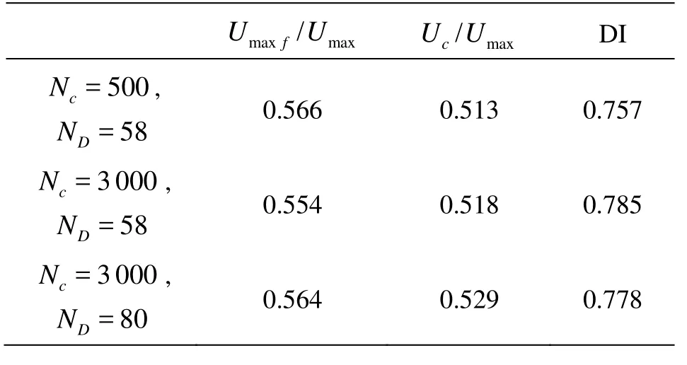
Table 1 Comparison of the meshes at T=15.0

Fig.2 Shapes of RBCs for different Capillary numbers. The solid lines are the results from Ref.[15], where the corresponding Capillary numbers are 0.05, 0.101, and 0.203, respectively

Zhao et al.[15]simulated the RBCs flowing through a narrow cylindrical tube using the boundary integral method. For comparison and validation, we employ the same geometry configuration. The diameter of the tube is 9.02 μm. The periodic boundary conditions are imposed at the inlet and the outlet, The distance between two neighboring cells is 2a, Fig.2 shows that our results are in a good agreement with previous studies.

2.2 One cell

In this section, the cells are aligned at an equal distance along the capillary. The computation domain is a periodic box as the part enclosed by the dash line in Fig.1. So only one cell is involved in the simulation and L=lc. In the present configuration, the volume fraction of the cell only depends on lc. The Capillary number and the Reynolds number based on Umaxare kept to be 0.69 and 0.72, respectively. Figure 3(a) shows the contour of the axial velocity on the X- Y symmetric plane with the tube length L=17.45a after the stable motion of the cell is reached. The velocity profiles on the two cross section planes, where the location 0 is the plane across the cell centroid and the locations 1, 2, 3 are L/12, L/6, L/2 from the location 0, respectively, as shown in Fig.3(b). If the volume fraction is small enough, there are two typical axial flow velocity profiles. One is the velocity profile far from the cell, for example, at the locations 2 and 3, which is very similar to the undisturbed parabolic profile without the RBC except that the maximum value is smaller. The other is the profile near the cell. Due to the existence of the cell, it can be seen that the velocity in the cell is almost identical to the platform in the plot of the velocity profile and the shear rate is increased in the gap between the cell and the wall. In the vicinity of the cell, the axial flow velocity is reduced which is also found in the plot of the axial velocity along the flow direction in Fig.3(c). These two kinds of modification of the flow are due to the introduction of cells, and according to the intensity of the influence of the cells, we can classify the hydrodynamic interactions among the cells into two types: the long-range interaction and the short-range interaction. The primary estimation of the radius short-range interaction can be performed according to Fig.3(c). If we define the criterion of the short-range interaction is the location where the axial velocity recovers to 99% of the maximum, the radius is about 3a-5a from the surface of the cell.

The long-range interaction is relative weak. In the dilute suspension, the main effect of the cells is on the rheology property of the suspension. The local properties, such as the shape of the cell, have little influence on the flow. The interaction between the cells and the suspending fluid is important. Figure 4 shows the mean axial velocity according to the cell volume fraction and it is indicated that the mean velocity decreases with the increase of the cell volume fraction, which implies that the introduction of the cells increases the apparent viscosity of the suspension, defined as

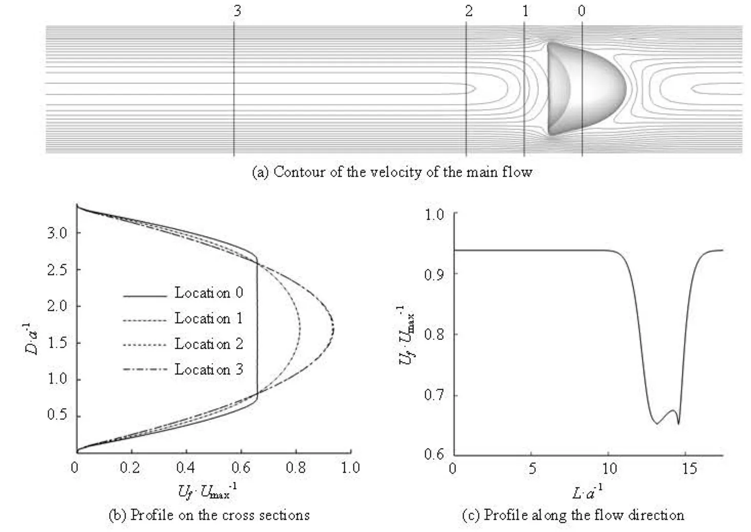
Fig.3 X-component of the flow

Fig.4 Mean flow velocity at different volume fraction of RBC

Fig.5 Velocity profiles on the selected cross section planes

For the short-range interaction, the local properties are important. As shown in Fig.3(a), the cell is deformed into a parachute-like shape and the distribution of the axial velocity in the vicinity of the cell depends on the cell shape. In Fig.3(c), the curve before the cell is steeper than that after the cell because the rear part is concaved, which makes the material points on the rear part surround the fluid nearby along the tube axis and have stronger influence. Figure 5 shows the short-range influence. The locations with the maximum values of the stream-wise velocity along the capillary axis are selected where the short-range interaction can be thought to be the weakest approximately. As the cell fraction increases, the short-range interaction becomes dominating and the parabolic-like profile becomes flat and then disappears, but the maximum value does not appear on the symmetric axis in the case of lc=2.91a.

With respect to the influence of the flow on the cell deformation, the distribution of the membrane material points in the flow field is important. For simplicity, we divide the membrane into the front part with the direction along the flow direction and the rear part with the adverse direction of the flow. For both parts, the material points near the wall move slower than those near the tube axis. The two parts are both transformed into a concave shape, but because of the membrane force, the concave degrees are different. With respect to the cell, the front part is protruded and the rear part is recessed. The difference of the axial velocity on the membrane causes the cell elongated. Actually, the deformation index is a parameter measuring the degree of the cell elongation and is determi-ned by the flow velocity profile. As shown in Fig.6, the deformation index increases with the decrease of the cell volume fraction but the key role is the flow velocity profile. From the mechanism of cell deformation, it can be seen that there are two factors to affect the cell deformation. One is the mean flow velocity, which determines the order of the global shear rate. The larger the flow velocity, the larger the cell elongation will be. The other is the shape of the velocity profile, which determines the velocity distribution on the membrane. The short-range interaction affects both factors, however, the long-range interaction’s effect is relatively smaller.

Fig.6 Deformation index for different volume fractions of RBC

Fig.7 Principal strain along the profile of the cell membrane

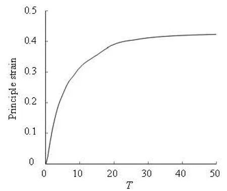
Fig.8 Development of the maximum principal strain

The absolute value of the principal strain is used to measure the local deformation. A cell in a long tube (L=17a) is taken as an example. Because the flow and the deformation are axi-symmetrical, only the strain along the half of the profile of the membrane is shown in Fig.7, where the difference of the vertical coordinate between the two curves denotes the value of the strain. It is found that on the concave rear part of the cell, the strain is small. On the front part, the maximum strain occurs on the middle location. The evolution of the maximum principal strain is also shown in Fig.8, which indicates that the principal strain increases as the deformation develops and reaches the maximum value when the cell is transformed into a steady shape.

2.3 A group of cells

In this section, the cells are distributed at an equal distance along the tube. The periodic computation domain contains a group of cells with an equal distance lc=1.94a between the neighboring cells, but the length of the domain L≠nlcwhere n is the number of the cells. From the analysis in the above section, it is known that each cell is placed in the short-range interactive domain of its neighboring cell. For the convenience of presentation, we name the leading cell in the flow direction as Cell 0, the next as Cell 1, and so on in the sequence. The Capillary number and the Reynolds number based on Umaxare still kept to be 0.69 and 0.72, respectively. The volume fraction is now determined by lcand L.

Figure 9 shows the series of snapshots of the cells and the contours of the axial velocity for the cell volume fraction of 8.34% at different instants. Four cells are involved in the simulation. It is obvious that the leading cell and the trailing cell do not have the short-range interaction from the front and back domains, respectively. The two middle cells have strong cell-cell interaction on both front and rear parts. The shapes of all cells are transformed from biconcave to parachute shapes. The equally distributed cells at the initial instant spread and repel each other along the flow direction. The gaps between each cell are not equal any more. All the gaps increase with the fastest growth between Cell 0 and Cell 1.

The tendency can be explained by the cell-cell hydrodynamic interaction. As revealed in Section 2.2, the velocity profile in the effective area of the shortrange interaction is more in the flat side and the peak value is smaller than that without the short-range influence. Compared to the other three cells, the front part of the leading cell with less short-range interaction, has higher speed and is sharper. The cell is more elongated, as indicated in the DI-time relations in Fig.10, which means that the whole cell is in the relatively high speed domain in the flow and runs faster than the others. Moreover, such influence is transferrred from cell to cell. Figure 11 shows the evolution ofthe relative velocities. The velocity of Cell i relative to Cell j is defined as

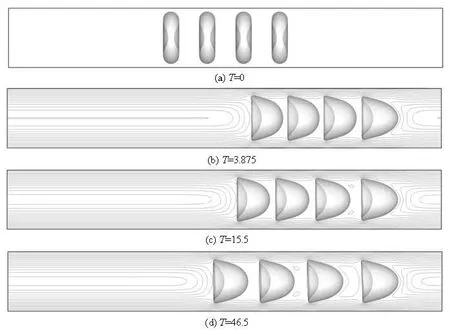
Fig.9 Series of the snapshots of the cells at different time

where subscript ci denotes the cell serial number. A similar phenomena and mechanism could be found in the following cells. For example, with respect to Cell 1, Uc1-0is larger than Uc2-1in the most of the time, which leads to a larger gap between Cell 1 and Cell 0 than that between Cell 2 and Cell 1. The short-range interaction of the Cell 1-Cell 0 pair is weak than that of Cell 2-Cell 1 pair and the consequent effects are DIc1＞DIc 2and Cell 1 moves faster than Cell 2 as shown by a similar analysis on Cell 0. The relative velocity shown in Fig.11 indicates that the cells are separated from each other in the current configuration.

Fig.10 DI vs. time

During the initial stage, the cells are driven and accelerated by the flow, the relative velocity increases disregarding the increment of the interactive distance. After that stage, the relative velocity, especially Uc1-0, decreases quickly. After about t=30, because of the difference of the relative interactive distance, Uc1-0drops to Uc2-1and Uc2-1, which implies that the shortrange effect vanishes quickly.

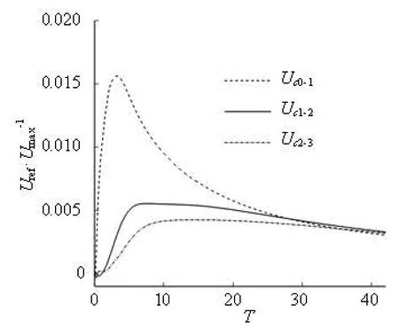
Fig.11 Relative velocity of the cell pairs

From Fig.11, we can also deduce that the leading cell obtains the highest translation velocity. Although there is no cell following the trailing cell and the rear part of the trailing cell is closer to the high speed domain of the flow with less short-range interaction than the other cells, its translation velocity is the lowest.

We also compute the cases of two and three cells with the same volume fraction to study the short-range interaction. Similar to the case of four cells, the cellsassume a parachute-like shape and repel each other. But there are some differences. The evolutions of the deformation index in all three cases are shown in Fig.12, where the same line represents the same case and the same symbol denotes the cell with the same location in the queue of the cell. It is interesting to note that DIs of Cell 0 are almost identical in all cases and the same tendency occurs for Cell 1 in the cases of two and three cells. In these two cases, the same thing is that their location in the cell queue and the situation about their neighboring cells which determines the short-range interaction. For Cell 0, there are cells after it and no cell before it. For Cell 1, there are cells before and after it. However, we also notice that a same distribution occurs to the last cell and its neighboring cell, except the relation of the directions of the flow and the cell motion. The fact is that the DI of Cell 0 is almost the same disregarding the number of the following cells, on the other hand, the DI of the last cell is highly dependent on the cells before it. So it might be deduced that the response of DI of cells to the short-range interaction are not even in all directions. The interaction to the front part of the cell has the priority to the elongation of the cell. But the difference of DI of Cell 2 between the cases of three and four cells shows that the short-range interaction, even for the rear part, still has a great effect on the deformation of the cell. Figure 12 also shows that the differences of the DI of the cell with the same serial number become smaller with the time. From Fig.9, which shows that the distance between the neighboring cells is growing, it is indicated that the short-range interactions diminish quickly as the range increases.

Fig.12 DI-time relations in the three cases

3. Conclusions

In this paper, the multi-cell hydrodynamic interactions in a micro tube with some special configurations of the flow and the cells are investigated. The hydrodynamic interactions can be classified into the long-rang interaction and the short-range interaction. The long-range interactions mainly affect the rheology properties of the suspension, change little the shape of the flow velocity profile and maybe have less sensitivity on the shape of the cell. The short-range interactions highly depend on the shape of the cell and the intensity is stronger, but the effective domain is limited to the vicinity of the cell. The short-range interactions modify the flow greatly on both the peak value and the profile shape. The shape of the cell is determined by the local profile of the background flow field. The fluid flow and the cells affect each other.

In the current configuration, the hydrodynamic interactions make the cells repel each other along the tube. The hydrodynamic interactions for the front part of the cell make more significant modification on the shape than that for the rear part.

In future work, more general configuration will be taken into account and the molecular scale cell-cell interaction will be considered.

[1] ZHU C., YAGO T. and LOU J. et al. Mechanisms for flow-enhanced cell adhesion[J].Annals of BiomedicalEngineering,2008, 36(4): 604-621.

[2] KHSMATULLIN D. B., TRUSKEY G. A. Three-dimensional numerical simulation of receptor-mediated leukocyte adhesion to surfaces: effects of cell deformability and viscoelasticity[J].Physics of Fluids,2005, 17: 031505.

[3] FISCHER T. M. Tank-tread frequency of the red cell membrane: Dependence on the viscosity of the suspending medium[J].Biophysical Journal,2007, 93(7): 2553-2561.

[4] NOGUCHI H. Swinging and synchronized rotations of red blood cells in simple shear flow[J].Physical Re-view E, 2009, 80(2): 021902.

[5] ZHANG J., JOHNSON P. C. and POPEL A. S. Red blood cell aggregation and dissociation in shear flows simulated by lattice Boltzmann method[J].Journal ofBiomechanics, 2008, 41(1): 47-55.

[6] SHI L., PAN T-W. and GLOWINSINSKI R. Deformation of a single red blood cell in bounded Poiseuille flows[J].Physical Review E, 2012, 85(1): 016307.

[7] AIDUN C. K., CLAUSEN J. R. Lattice Boltzmann method for complex flows[J].Annual Review of FluidMechanics,2010, 42: 439-472.

[8] DUARTE F., GORMAZ R. and NATESAN S. Arbitrary Lagrangian-Eulerian method for Navier-Stokes equations with moving boundaries[J].Computer Methods in Applied Mechanics and Engineering,2004, 193: 4819-4836.

[9] POZRIDIS C. Axisymmetric motion of a file of red blood cells through capillaries[J],Physics of Fluids,2005, 17(3): 031503.

[10] ANDERSON W. An immersed boundary method wall model for high-Reynolds-number channel flow over complex topography[J].International Journal for Numerical Methods in Fluid,2013, 71(12): 1588- 1608.

[11] LIU Y., LIU W. K. Rheology of red blood cell aggregation by computer simulation[J].Journal of Compu-tational Physics,2006, 220(1): 139-154.

[12] BAAIJENS F. P. T. A fictitious domain/mortar element method for fluid-structure interaction[J].InternationalJournal for Numerical Methods in Fluid,2001, 35(7): 743-761.

[13] ZHANG J., JOHNSON P. C. and POEL A. S. Effects of erythrocyte deformability and aggregation on the cell free layer and apparent viscosity of microscopic blood flows[J].Microvascular Research,2009, 77(3): 265- 272.

[14] YE T., LI H. and LAM K. Y. Modeling and simulation of microfluid effects on deformation behavior of a red blood cell in a capillary[J].Microvascular Research,2010, 80(3): 453-463.

[15] ZHAO H., ISFAHANI A. H. G. and OLSON L. N. et al. A spectral boundary integral method for flowing blood cells[J].Journal of Computational Physics,2010, 229(10): 3726-3744.

[16] SHI X., LIM S. P. A LBM-DLM/FD method for 3D fluid-structure interactions[J]Journal of Computatio-nal Physics,2007, 226(2): 2028-2043.

[17] FUNG Y. C.Biomechanics: mechanical properties of living tissues[M]. 2nd Edition, New York, USA: Springer-Verlag, 1993.

[18] TSUKADA K., SEKIZUKA E. and OSHIO C. Direct measurement of erythrocyte deformability in diabetes mellitus with transparent microchannel capillary model and high-speed video camera system[J].MicrovascularResearch,2001, 61(3): 231-239.

[19] LI J., DAO M. and LIM C. T. et al. Spectrin-level modeling of the cytoskeleton and optical tweezers stretching of the erythrocyte[J].Biophysical Journal,2005, 88(5): 3707-3719.

[20] FEDOSOV D., CASWELLl B. and KARNIADAKIS G. E. A multiscale red blood cell model with accurate mechanics, rheology, and dynamics[J].Biophysical Jour-nal,2010, 98(10): 2215-2225.

[21] YU Z. A DLM/FD method for fluid/flexible-body interactions[J].Journal of Computational Physics,2005, 207(1): 1-27.

[22] NOURGALIEV R. R., DINH T. N. and THEOFANOUS T. G. et al. The lattice Boltzmann equation method: Theoretical interpretation, numerics and implications[J].International Journal of Multiphase Flow,2003, 29(1): 117-169.

10.1016/S1001-6058(14)60020-2

* Project supported by the National Natural Science Foundation of China (Grant Nos. 11372278, 10902098), the Fundamental Research Funds of the Central Universities (Grant No. 2010QNA40107).

Biography: SHI Xing (1975-), Male, Ph. D., Associate Professor

ZHANG Shuai, E-mail: shuaizhang@zju.edu.cn