
A Piecewise Modeling Approach for Climate Sensitivity Studies:Tests with a Shallow-Water Model
2015-11-21 11:23SHAOAimei邵爱梅QIUChongjian邱崇践andNIUGuoYue
SHAO Aimei(邵爱梅),QIU Chongjian(邱崇践),and NIU Guo-Yue
1 Key Laboratory for Semi-Arid Climate Change of the Ministry of Education,College of Atmospheric Sciences,Lanzhou University,Lanzhou 730000,China
2 Department of Hydrology and Water Resources,University of Arizona,Tucson,AZ 85721,USA
3 Biosphere 2,University of Arizona,Tucson,AZ 85738,USA
A Piecewise Modeling Approach for Climate Sensitivity Studies:Tests with a Shallow-Water Model
SHAO Aimei1∗(邵爱梅),QIU Chongjian1(邱崇践),and NIU Guo-Yue2,3
1 Key Laboratory for Semi-Arid Climate Change of the Ministry of Education,College of Atmospheric Sciences,Lanzhou University,Lanzhou 730000,China
2 Department of Hydrology and Water Resources,University of Arizona,Tucson,AZ 85721,USA
3 Biosphere 2,University of Arizona,Tucson,AZ 85738,USA
In model-based climate sensitivity studies,model errors may grow during continuous long-term integrations in both the“reference”and“perturbed”states and hence the climate sensitivity(defined as the difference between the two states).To reduce the errors,we propose a piecewise modeling approach that splits the continuous long-term simulation into subintervals of sequential short-term simulations,and updates the modeled states through re-initialization at the end of each subinterval.In the re-initialization processes,this approach updates the
tate with analysis data and updates the perturbed states with the sum of analysis data and the difference between the perturbed and the reference states,thereby improving the credibility of the modeled climate sensitivity.We conducted a series of experiments with a shallow-water model to evaluate the advantages of the piecewise approach over the conventional continuous modeling approach.We then investigated the impacts of analysis data error and subinterval length used in the piecewise approach on the simulations of the reference and perturbed states as well as the resulting climate sensitivity.The experiments show that the piecewise approach reduces the errors produced by the conventional continuous modeling approach,more effectively when the analysis data error becomes smaller and the subinterval length is shorter.In addition,we employed a nudging assimilation technique to solve possible spin-up problems caused by re-initializations by using analysis data that contain inconsistent errors between mass and velocity.The nudging technique can effectively diminish the spin-up problem,resulting in a higher modeling skill.
climate sensitivity,modeling approach,nudging technique,model uncertainty
1.Introduction
Model-based climate sensitivity studies facilitate isolating the impact of an individual external forcing on climate change and extreme weathers from other forcings.They have been extensively used to identify the major causes of the observed climate anomaly by differentiating various anthropogenic forcings(e.g.,greenhouse gas emissions,land use and land cover changes,etc.)from natural forcings(e.g.,volcanic eruptions,changes in solar output,etc.)that together contribute to historical and present climate changes(e.g.,Meehl et al.,1996,2000;Santer et al.,1996,2003;Wei et al.,2012;Dong et al.,2014).In addition,they have been used to diagnose possible influences of anomalous external forcings(e.g.,ocean temperature,ice and snow cover,soil moisture,etc.)on extreme weathers(e.g.,Huang et al.,2006;Zhou and Yu,2006;Kim and Hong,2007;Li et al.,2007;Lian et al.,2009;Seol and Hong,2009;Mohino et al.,2011;Peings et al.,2012;Notaro et al.,2013;Vavrus et al.,2013;Peings and Magnusdottir,2014;Wang et al.,2015).These model sensitivity studies require to run a model at least twice:a“control run”and a“perturbation run”.The control run simulates the historical or present atmospheric state as realistic as possible while considering as many forcings as possible,producing a“reference state”. The perturbation runs with an(or several)individual external forcing(s)being modified(while others being fixed)produce hypothetical atmospheric states or“perturbed states”.The averaged differences between the perturbed states and reference state over a long period are then regarded as climate sensitivities to(or the climatic impact of)the modified external forcing(s).The credibility of the climate sensitivity depends on the accuracy of these model simulations,although model errors may be partially offset in the differences between reference and perturbed states.
Supported by the National Natural Science Foundation of China(41330527 and 41275102),Fundamental Research Funds for the Central Universities(lzujbky-2013-k16),and Program for New Century Excellent Talents in Universities(NCET-11-0213).
∗Corresponding author:sam@lzu.edu.cn.
©The Chinese Meteorological Society and Springer-Verlag Berlin Heidelberg 2015
Through decades of development,state-of-the-art climate models are still problematic to accurately simulate climate dynamics due mainly to the nonlinearity of the atmospheric dynamics as well as the interactions between various components of the complex climate system.As such,model errors may grow during continuous long-term integrations of both the reference and perturbed climates,decreasing the credibility of the modeled climate sensitivity(Stainforth et al.,2005;Douglass et al.,2008;Klocke et al.,2011;Sanderson,2011).Improving the realism of the models'dynamics and physics is undoubtedly a pathway,but a daunting task,for enhancing the credibility of the sensitivity studies.In this study,we explore alternative ways to reduce the model errors by improving simulation approach on the basis of existing models.
In dynamical climate downscaling,many researchers have used atmospheric reanalysis data or general circulation models'(GCMs)outputs to constrain their simulations through re-initialization(Qian et al.,2003)or nudging(von Storch et al.,2000;Lo et al.,2008;Harkey and Holloway,2013).Their results suggested that re-initialization or nudging mitigates accumulation of systematic errors in the continuous long-term simulations,producing better downscaling results(Lo et al.,2008).Analogous to the downscaling,in this study,we attempt to use historical data to constrain all simulated states,including the reference field and the perturbed field.Because there was no such data for the perturbed states,we proposed a piecewise modeling approach to solve this dilemma(Zhang et al.,2008).For the reference state,the approach is similar to the conventional re-initialization that divides the entire integration period into a number of subintervals for a series of sequential short-term simulations,and at the end of each subinterval,the simulated fields are updated with analysis data.For the perturbed states,the approach is different from the conventional re-initialization,the data used for updating the simulated fields are the sum of the analysis and the difference between the perturbed and reference states.In such a way,the resulting climate sensitivity to changes in the external forcing can be improved with greater credibility.We tested the approach with a simple six-parameter model,and the preliminary results indicated that the approach is able to effectively correct the drifts of the modeled climates,resulting in higher model accuracy(Zhang et al.,2008).However,the model was too simple with a very low degree of freedom,and the experiments designed were too specific.In this study,we will more comprehensively assess the performance of the piecewise approach and its applicability under broader scenarios through experiments with the shallow-water model.The focus of this study is on assessing the influence of the analysis data error and subinterval length on the simulation skill.We also explore ways to mitigate the spin-up problems caused by frequent re-initializations.
2.The piecewise simulation approach and nudging technique
2.1 The piecewise simulation approach
For simplicity,a climate model can be expressed as
where F(x)is the model forcing terms,x is model prognostic variable,and x0is its initial state.Conventionally,the model is integrated in a continuous way from time t=t0to time t=TNto produce a simulated atmospheric state that evolves with timeunder forcings F(x).For climate sensitivity studies,the above model should be run at least twice with different external forcings.The first run with actual forcings Fr(x),named as a control run,produces a reference state,xr.The conventional continuous integration can be written as
where Δt is the time step size,and subscript n represents the number of time steps.The other run with modified forcings Fp(x)produces a perturbed state,xp:
Subtracting Eq.(2)from Eq.(3)results in the difference between the two states:

The averaged difference over a long period is then defined as climate sensitivity,which is regarded as the effects of the modified forcings.Conventionally,both the reference and the perturbed states are obtained through the above continuous long-term model integrations. To improve the realism of the modeled climate,the reference state,in particular,can be constrained with the observations or analysis data through nudging or re-initialization,when observations or analysis data are available for the reference state.However,the perturbed state is produced as a result from free model integration without any constraint for lack of such data.For this reason,reanalysis or observations have rarely been used in climate sensitivity studies.In the followings,we present a piecewise method,through which analysis data(including reanalysis)can be introduced to constrain not only the reference state but also the perturbed state to improve the simulation accuracy.
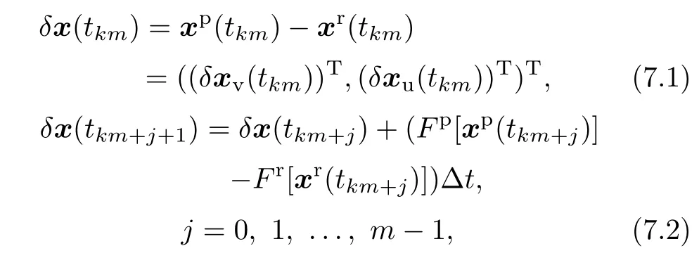
In the piecewise approach,the entire integration period(NΔt)is divided into a number of short-term subintervals,whose lengths are σ=mΔt(m<<N);at the end of each subinterval,the modeled states are then updated with the analysis.Considering that the analysis is usually not available for all the prognostic variables,we separate the prognostic variables into two categories:xr=((xrv)T,(xru)T)T,where xrvrepresents the variables that are available,xrurepresents the variables that are not available in the analysis,and the superscript T denotes transpose of a matrix.In such a case,only xrvis updated,while xruremains unchanged. For the kth subinterval(from t=tkmto t=t(k+1)m)the reference state can be written initially as
and subsequently,

The perturbed state is updated with the sum of the analysis and the difference between the reference and the perturbed state,at the end of each subinterval,kmΔt:

Subtracting Eq.(5.1)from Eq.(6.1)and Eq.(5.2)from Eq.(6.2)results in the difference between the reference and perturbed states at times km and km+j+1,respectively:
2.2 Nudging technique
A major concern when applying the piecewise simulation method is whether the simulated state as represented by the analysis data that are used in the re-initialization deviates significantly from the modeled state,inducing a“spin-up”problem.To avoid the possible spin-up problem,we use the Newtonian relaxation or“nudging”assimilation techniques to“reassimilate”the original analysis data to the piecewise runs.The nudging method(Charney et al.,1969;Hoke and Anthes,1976;Stauffer and Seaman,1990)has been extensively used in data assimilation for numerical weather prediction,dynamical downscaling(von Storch et al.,2000;Lo et al.2008;Salameh et al.,2010;Harkey and Holloway,2013),and estimating and correcting model errors of global circulation models(Danforth et al.,2007).The nudging method relaxes the model states toward the observed states by adding an artificial tendency based on the difference between the two.Following Stauffer and Seaman(1990),the nudging can be expressed as:

where x is the modeled state,andˆx is the corresponding observational state(in our experiments it is actually the analysis data);F represents the forcings,wta temporal weight,and εxa quality factor,which ranges between 0 and 1 depending on the accuracy of the observational data(εx=1 for all variables in this study).Following Stauffer and Seaman(1990),the nudging factor Gx=3×10⁻⁴s-1for all the prognostic variables,and the temporal weighting function is
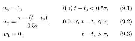
where t is time,tsis the time of the analysis data,and τ is a predetermined time window over which the analysis data affect the model simulation and in our experiments τ=6 h.The nudging run re-assimilates the original analysis data to obtain new analysis data for updating the reference and the perturbed states at the end of each subinterval(Fig.1).
3.Model and experimental design
3.1 The shallow-water model
The two-dimensional shallow-water model with the f-plane with rolling bottom is used to test the piecewise method.The prognostic equations are:

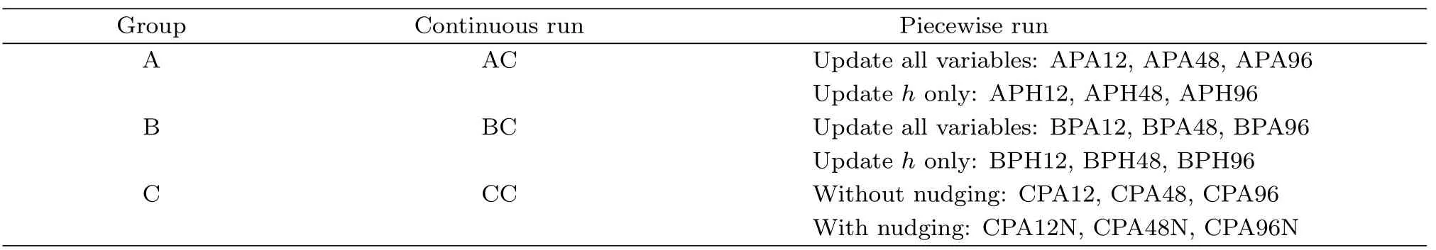
where u and v represent the current velocity at x and y directions,respectively;h the perturbation height;f the Coriolis parameter;H (=3000 m)the basic depth;and hsthe terrain height,which is set up as a circular cone at the center of the model domain with a radius of 12 grids.The maximum terrain height hsmaxis 120 m for the“perfect”model and 105 m for the“imperfect”model in the following experiments.The model domain is specified as a 61×61 domain with agrid spacing of 200 km(a relatively coarse resolution to maintain computational stability).Periodic boundary conditions are used,and the time step size Δt is 60 s. The initial perturbation height is shown in Fig.2,and the initial velocity is given as a result of geostrophic balance.The model runs for 90 days.
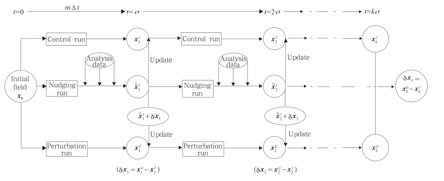
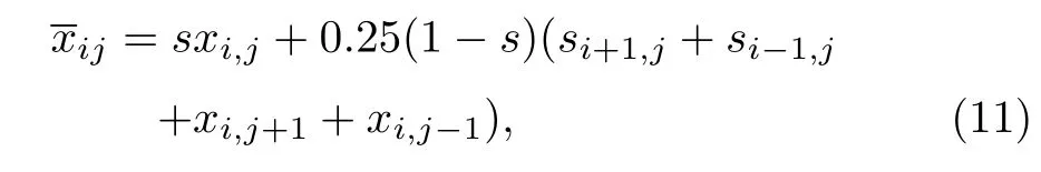
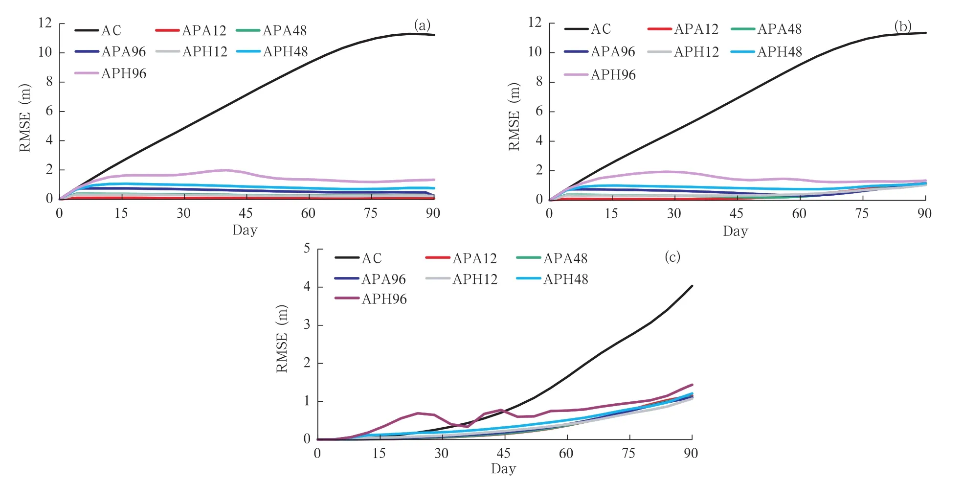
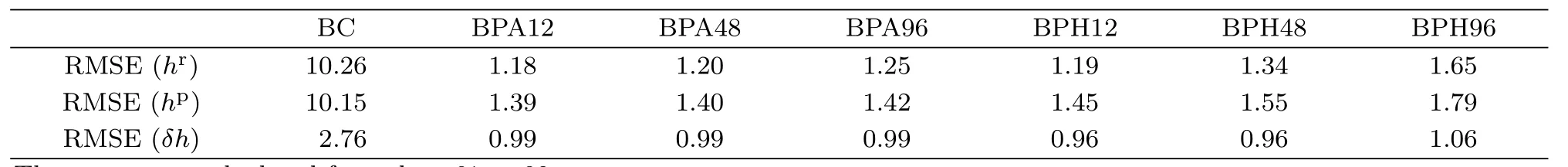
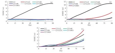
Fig.1.Computational flow chart of the piecewise approach with nudging.The entire integration period(NΔt)is divided into a number of short-term subintervals,whose lengths are σ=mΔt(m< 3.2 Experimental design The experiments are designed to assess the effect of the modified Coriolis parameter f on predictions of the height.The control run is conducted with a linearly increasing f with time from 1.0×10⁻⁴to 1.2 ×10⁻⁴s-1at the end of the simulations,while the perturbation run is conducted with f as a constant of 1.0×10⁻⁴s-1.The reference state of height hr(resulting from the control run with perfect model)and δh(the difference between the control and perturbation runs with the perfect model,of which hsmax=120 m),are regarded as the“truth”and used to evaluate the imperfect model,of which hsmax=105 m.As a result from the continuous long-term simulations(the control and perturbation runs),the standard deviation(STD)of δh from the perfect model increases steadily and reaches a maximum of 7.07 m by the end of the simulations,and the root mean square error(RMSE) of hrand hpfrom the imperfect model increases to a maximum of about 11.3 m on day 84(Fig.3).This suggests that the impact of model error on the simulation accuracy exceeds that of the modified forcings in the following experiments. Two key factors affecting the simulations of the piecewise approach are the length of the subinterval and data quality including the number of analysis vari-ables and data accuracy.To examine the impacts of these two factors on the simulations,we design the following three groups of experiments,in which the analysis data with different error levels are used. Fig.2.The initial perturbation height and wind.The contour interval is 20 m for the perturbation height.The vectors are for the wind,and the vector scale(10 m s-1)is labeled at the bottom of the panel. Fig.3.Temporal variations of the root mean square error(RMSE)of the reference state hrand the perturbed state hpresulting from the runs with the“imperfect model”,and standard deviation(STD)of δh resulting from the runs with the“perfect model”(see definitions in the text). Group A:analysis data are perfect;the“true”states of h,u,and v produced by the perfect model are directly used as analysis data. Group B:analysis data contain consistent errors between height(h)and velocity(u and v);they are consistently produced as a result from iteratively smoothing the“truth”12 times through the following smoothing operators: where the subscripts i and j are grid point index at x and y directions,respectively,andis the result of smoothing.The smoothing factor s is equal to 0.5 for all the three variables.The domain-averaged RMSEs of the resulting analyses are 1.12 m for h,0.08 m s-1for u,and 0.12 m s-1for v,respectively,which are approximately equal to 7 times the error of the 24-h simulation with the initial fields(Fig.2). Group C:analysis data have inconsistent errors;the analysis of h is the same to that in Group B with a smoothing factor of 0.5,while the analyses of u and v result from iteratively smoothing the“truth”6 times with a smoothing factor of-0.25 in Eq.(11).The resulting domain-averaged RMSE decreases to 0.07 and 0.08 m s-1,respectively.Compared with Group B,the analysis of h has the same errors,but the errors in the analyses of u and v decrease.As such,the dynamic equilibrium in the analyses may be broken,because of the opposite smoothing factors that are applied to h,u,and v through Eq.(11).The inconsistence between height and velocity may lead to model spin-up problems.We then designed some experiments to examine the impacts of the spin-up problems on the simulation accuracy and the ability of the nudging technique to solve the spin-up problems. As shown in Table 1,each group of the experiments consists of one continuous simulation(denoted as C)and six simulations using the piecewise approach(P).In Groups A and B,three simulations are updated with all the variables(A),while the other three are updated with h only(H);the piecewise subintervals are 12,48,and 96 h,respectively.In Group C,all the six piecewise simulations are updated with all the three variables h,u,and v,and the piecewise subintervals are also 12,48,and 96 h,respectively.However,three simulations are with nudging(the analyses are obtained from the nudging assimilation,denoted as N),while the other three are without nudging. Table 1.List of the experiments 4.1 Group A experiments The errors of hrand hpfrom the continuous run(experiment AC)grow with time,but this growing feature disappears in all the six piecewise runs(Fig.4). The errors of hr,hp,and δh from the piecewise runs with updating of all the variables(APAs)are generally smaller than those with updating of h only(APHs). However,these errors increase with subinterval length for APHs.For instance,the piecewise runs with a smaller subinterval length(e.g.,12 or 48 h)perform better than those with a greater length(96 h),more obviously from days 15 to 45(Fig.4).The δh error resulting from APH96 exceeds the error from the continuous run AC in the first 30 days and becomes smaller after day 45(Fig.4c).The δh errors from the other five piecewise runs,which are close to each other,increase with time till the end of the simulation.Those δh errors are close to that from AC in the first 20 days but about 3 times smaller than that from AC by the end of the simulation period.Overall,the piecewise approach is superior to the continuous approach in such a case that no errors exist in the analysis data.The advantage of the piecewise approach over the continuous approach is more apparent for a longer integration,because the errors resulting from the piecewise control and perturbed runs are almost at the same level as those from AC on day 7,but much less afterwards. Table 2 lists the RMSE in averaged hr,hp,and δh over the last 30 days(from days 61 to 90)from the seven experiments of Group A,which means that the results are shown from a climate standpoint.The simulation errors produced by the six piecewise runs are much less than those by the continuous run.The errors of averaged hrincrease with subinterval length;these errors produced by the piecewise runs with updating of h only are about 2-3 times larger than those by the runs with updating of all the three variables. However,the errors of averaged hpdo not increase(even decrease)with subinterval length when all the three variables are updated simultaneously;but they increase with subinterval length when only h is updated.Generally,the errors of averaged hpare smaller when all the variables are updated,except for the run with a 12-h subinterval length(APA12),which produces an error slightly larger than does the run with updating of h only(APH12).The errors of averaged δh over the last 30 days produced by the piecewise runs are generally three times smaller than those by the continuous runs.For a longer subinterval length,e.g.,96 h,the piecewise approach prefers updating all the variables to updating h only.However,when less analysis variables(only h in this testing case)are available,a shorter piecewise subinterval(<48 h)is preferred. Fig.4.Temporal variations of the root mean square error(RMSE)of(a)reference state,(b)perturbed state,and(c)difference δh resulting from Group A experiments. Table 2.RMSE in averaged hr,hp,and δh from the seven experiments in Group A 4.2 Group B experiments The temporal variations of hr,hp,and δh errors resulting from the seven runs resemble those from Group A experiments,except that the errors of hrand hpresulting from the piecewise runs are larger than those from Group A because of the larger analysis data errors(figure omitted). Table 3 lists the RMSE of averaged hr,hp,and δh over the final 30 days.The error of the continuous run(BC)is slightly different from that of Group A(AC),indicating the continuous simulation is not very sensitive to the analysis data error.Although the errors of averaged hrand hpresulting from the six piecewise runs become larger,the error of averaged δh does not increase much,because the errors of averaged hrand hpmostly offset within the short subintervals in the piecewise runs.The impacts of the subinterval length and the number of updated variables on the simulation skill are similar to that of Group A.The errors from the six piecewise runs are also much less than that resulting from the continuous simulation even if greater errors exist in the analysis data. Table 3.RMSE in averaged hr,hp,and δh from the seven experiments in Group B 4.3 Group C experiments The errors of hrproduced by the six piecewise runs of Group C,are close to each other,and remain stably smaller than that by CC(Fig.5a).The errors of hpresulting from CPA12 grow more rapidly after day 45,becoming larger than those from CPA48 and CPA96(Fig.5b).However,when the nudging technique is applied,this situation disappears.The δh errors from the three runs with the nudging analysis are generally smaller than those without nudging,which differ significantly from each other(Fig.5c).Without nudging,the error produced by CPA12 exceeds that by CC after day 24,with a maximum error(5.37 m)being larger than that by CC(3.92 m).CPA48 performs much better than does CPA12,reaching a maximum of 2.52 m by the end.CPA96(though its error grows faster during the initial stage)performs better than CPA48 after day 44,reaching a maximum of 2.17 m by the end.This indicates that less frequent updating of the states with analysis data that contains inconsistent errors(between height and velocity)may result in a better model performance in simulating climate sensitivity,when no nudging is applied. Averaged over the last 30 days,the error of averaged hrfrom the three piecewise runs without nudging(CPA12,CPA48,and CPA96;listed in Table 4)is smaller than those from Group B(BPA12,BPA48,and BPA96)due likely to the fact that the analysis data error of u and v in Group C is smaller than that in Group B.However,the error of averaged hpfrom CPA12 is larger than that from BPA12 but decreases with increasing subinterval length(CPA48 and CPA96),indicating that less frequent updating is preferred in the case of inconsistent errors existing in the analysis data.However,the use of nudging techniquesignificantly reduces the errors of averaged hr,hp,and δh,which become smaller with a shorter subinterval length,indicating that more frequent updating is preferred when nudging is applied. Fig.5.As in Fig.4,but for Group C experiments. Table 4.RMSE in averaged hr,hp,and δh from the seven experiments in Group C Model-based climate sensitivity studies are powerful tools for studying the impact of modified external forcings on climate change and for understanding the mechanisms of climate anomaly.Usually,the sensitivity experiments require at least two simulations:one is conducted with as many external forcings as possible,resulting in a reference state;while the other with modified forcings,resulting in a perturbed state.The difference between the two states averaged over a long term is then regarded as the effect of the modified external forcings,or climate sensitivity.However,model errors may grow during the continuous long-term integrations in both the reference and perturbed climate states and hence the climate sensitivity. To reduce the errors,we propose a piecewise modeling approach that splits the continuous long-term simulation into a number of subintervals of sequential short-term simulations,and updates the modeled states through re-initialization at the end of each subinterval.Many researchers have already applied reinitialization or nudging in dynamical climate downscaling with regional climate models.Following these previous climate downscaling studies,the piecewise approach updates the reference state with the analysis data.Moreover,the piecewise approach further updates the perturbed states with the sum of analysis data and the difference between the perturbed and the reference states at the end of each subinterval,thereby improving the credibility of the modeled climate sensitivity. To investigate the impacts of analysis data errors and subinterval lengths on the simulation of climate sensitivity using the piecewise approach,we designedGroups A and B experiments with the shallow-water model,both with subinterval lengths varying from 12,48,to 96 h.The analysis data for updating the model states contain larger errors in Group B experiments than in Group A experiments.Considering analysis data availability,we also divide the experiments into two categories:updating with all variables and updating with only one variable.The conclusions with regard to the modeled climate sensitivity drawn from the experiments are as follows. 1)Errors produced by the piecewise approach is about 2-3 times smaller than those by the continuous approach under most cases,either with no or large analysis data errors,or updating one variable or more variables. 2)When fewer analysis variables are available,a shorter piecewise subinterval(<48 h)is preferred. For a larger piecewise subinterval(e.g.,96 h),the piecewise approach prefers updating all the variables to updating only one. To investigate the impact of the spin-up problems induced by inconsistent analysis data errors on the modeled climate sensitivity,we designed Group C experiments by employing opposite factors in the smoothing operator(-0.25 for velocity and 0.5 for height)to generate inconsistent analysis data errors. We also used a nudging assimilation technique to solve the spin-up problems.The conclusions drawn from Group C experiments and through comparing it with Groups A and B experiments are: 1)Inconsistent analysis data errors result in larger model errors but still are much smaller than the continuous approach in the case of nudging. 2)Without nudging,less frequent updating of the modeled states with analysis data that contain inconsistent errors may result in a better model performance. 3)The use of nudging technique significantly reduces the model errors and more frequent updating is preferred. The piecewise modeling approach is promising for climate sensitivity studies as evidenced from the above experiments with the shallow-water model.However,the simple model does not include a feedback mechanism,with which the change in climate states in response to changes in an external forcing may feed back to the external forcing.Therefore,the approach needs to be further tested with a more complex model with greater climatic realism.Furthermore,since the approach can be used only when the observations or analysis data are available for one of the simulated states,it cannot be used in the prediction of future climate. Acknowledgments.The authors thank Dr. Gao Jidong for insightful comments and suggestions. Charney,J.,M.Halem,and R.Jastrow,1969:Use of incomplete historical data to infer the present state of the atmosphere.J.Atmos.Sci.,26,1160-1163. Danforth,C.M.,E.Kalnay,and T.Miyoshi,2007:Estimating and correcting global weather model error. Mon. Wea. Rev.,135,281-299,doi:10.1175/MWR3289.1. Dong,L.,T.J.Zhou,and B.Wu,2014:Indian ocean warming during 1958-2004 simulated by a climate system model and its mechanism.Climate Dyn.,42,203-217,doi:10.1007/s00382-013-1722-z. Douglass,D.H.,J.R.Christy,B.D.Pearson,et al.,2008:A comparison of tropical temperature trends with model predictions.Int.J.Climatol.,28,1693-1701,doi:10.1002/joc.1651. Harkey,M.,and T.Holloway,2013:Constrained dynamical downscaling for assessment of climate impacts. J.Geophys. Res.,118,2136-2148,doi:10.1002/jgrd.50223. Hoke,J.E.,and R.A.Anthes,1976:The initialization of numerical models by a dynamic-initialization technique.Mon.Wea.Rev.,104,1551-1556. Huang Yanyan,Qian Yongfu,and Wan Qilin,2006:Simulation and analysis about the effects of geopotential height anomaly in tropical and subtropical region on droughts or floods in the Yangtze River valley and North China.Acta Meteor.Sinica,20,426-436. Kim,J.-E.,and S.-Y.Hong,2007:Impact of soil moisture anomalies on summer rainfall over East Asia:A regional climate model study.J.Climate,20,5732-5743,doi:10.1175/2006JCLI1358.1. Klocke,D.,P.Robert,and Q.Johannes,2011:On constraining estimates of climate sensitivity withpresent-day observations through model weighting. J.Climate,24,6092-6099. Li Qiaoping,Ding Yihui,and Dong Weijie,2007:A numerical simulation study of impacts of historical land-use changes on the regional climate in China since 1700.Acta Meteor.Sinica,21,9-23. Lian Lishu,Shu Jiong,and Li Chaoyi,2009:The impacts of grassland degradation on regional climate over the origin area of three rivers in Qinghai-Tibetan Plateau,China.Acta Meteor.Sinica,67,580-590.(in Chinese) Lo,J.C.-F.,Z.L.Yang,and R.A.Pielke Sr.,2008:Assessment of three dynamical climate downscaling methods using the weather research and forecasting(WRF)model.J.Geophys.Res.,113,D09112,doi:10.1029/2007JD009216. Meehl,G.A.,W.M.Washington,D.J.Erickson III,et al.,1996:Climate change from increased CO2and the direct and indirect effects of sulfate aerosols. Geophys.Res.Lett.,23,3755-3758. Meehl,G.A.,W.M.Washington,J.M.Arblaster,et al.,2000:Anthropogenic forcing and decadal climate variability in sensitivity experiments of twentiethand twenty-first-century climate.J.Climate,13,3728-3744. Mohino,E.,B.Rodr´ıguez-Fonseca,C.R.Mechoso,et al.,2011:Impacts of the tropical Pacific/Indian oceans on the seasonal cycle of the West African monsoon.J.Climate,24,3878-3891,doi:10.1175/ 02011JCLI3988.1. Notaro,M.,K.Holman,A.Zarrin,et al.,2013:Influence of the Laurentian Great Lakes on regional climate. J.Climate,26,789-804,doi:10.1175/JCLI-D-12-00140.1. Peings,Y.,D.Saint-Martin,and H.Douville,2012:A numerical sensitivity study of the influence of Siberian snow on the northern annular mode.J.Climate,25,592-607,doi:10.1175/JCLI-D-11-00038.1. Peings,Y.,and G.Magnusdottir,2014:Role of sea surface temperature,Arctic sea ice and Siberian snow in forcing the atmospheric circulation in winter of 2012-2013.Climate Dyn.,doi:10.1007/s00382-014-2368-1. Qian,J.H.,A.Seth,and S.Zebiak,2003:Reinitialized versus continuous simulations for regional climate downscaling.Mon.Wea.Rev.,131,2857-2874. Salameh,T.,P.Drobinski,and T.Dubos,2010:The effect of indiscriminate nudging time on large and small scales in regional climate modelling:Application to the Mediterranean basin.Quart.J.Roy. Meteor.Soc.,136,170-182,doi:10.1002/qj.518. Sanderson,B.M.,2011:A multimodel study of parametric uncertainty in predictions of climate response to rising greenhouse gas concentrations.J.Climate,24,1362-1377,doi:10.1175/2010JCLI3498.1. Santer,B.D.,K.E.Taylor,T.M.L.Wigley,et al.,1996:A search for human influences on the thermal structure of the atmosphere.Nature,382,39-46,doi:10.1038/382039a0. Santer,B.D.,M.F.Wehner,T.M.L.Wigley,et al.,2003:Contributions of anthropogenic and natural forcing to recent tropopause height changes.Science,301,479-483. Seol,K.-H.,and S.-Y.Hong,2009:Relationship between the Tibetan snow in spring and the East Asian summer monsoon in 2003:A global and regional modeling study.J.Climate,22,2095-2110. Stainforth,D.A.,T.Aina,C.Christensen,et al.,2005:Uncertainty in predictions of the climate response to rising levels of greenhouse gases.Nature,433,403-406,doi:10.1038/nature03301. Stauffer,D.R.,and N.L.Seaman,1990: Use of four-dimensional data assimilation in a limitedarea mesoscale model.Part I:Experiments with synoptic-scale data.Mon.Wea.Rev.,118,1250-1277. Vavrus,S.,M.Notaro,and A.Zarrin,2013:The role of ice cover in heavy lake-effect snowstorms over the Great Lakes basin as simulated by RegCM4.Mon. Wea.Rev.,141,148-165,doi:10.1175/MWR-D-12-00107.1. Von Storch,H.,H.Langenberg,and F.Feser,2000:A spectral nudging technique for dynamical downscaling purposes.Mon.Wea.Rev.,128,3664-3673. Wang Die,Miao Junfeng,and Zhang Da-Lin,2015:Numerical simulations of local circulation and its response to land cover changes over the Yellow Mountains of China.J.Meteor.Res.,29,667-681,doi:10.1007/s13351-015-4070-6. Wei,T.,S.L.Yang,J.C.Moore,et al.,2012:Developed and developing world responsibilities for historical climate change and CO2mitigation.Proc.Natl. Acad.Sci.USA.,109,12911-12915. ˘Zagar,N.,M.˘Zagar,J.Cedilnik,et al.,2006:Validation of mesoscale low-level winds obtained bydynamical downscaling of ERA40 over complex terrain.Tellus A,58,445-455,doi:10.1111/j.1600-0870.2006.00186.x. Zhang Zhifu,Qiu Chongjian,and Wang Chenghai,2008:A piecewise-integration method for simulating the influence of external forcing on climate.Prog.Nat. Sci.,18,1239-1247. Zhou,T.J.,and R.C.Yu,2006:Twentieth-century surface air temperature over China and the globe simulated by coupled climate models.J.Climate,19,5843-5858,doi:10.1175/JCLI3952.1. Shao Aimei,Qiu Chongjian,and Niu Guo-Yue,2015:A piecewise modeling approach for climate sensitivity studies:Tests with a shallow-water model.J.Meteor.Res.,29(5),735-746, 10.1-007/s13351-015-5026-6. (Received March 11,2015;in final form August 19,2015)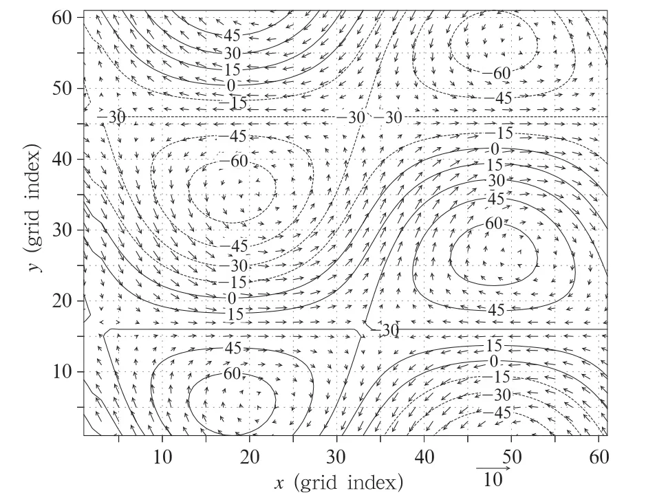

4.Results


5.Conclusions
 Journal of Meteorological Research2015年5期
- Journal of Meteorological Research的其它文章
- Interannual Variability of the Wintertime Northern Branch High Ridge in the Subtropical Westerlies and Its Relationship with Winter Climate in China
- Analysis of Tibetan Plateau Vortex Activities Using ERA-Interim Data for the Period 1979-2013
- Characteristics and Mechanisms of the Sudden Warming Events in the Nocturnal Atmospheric Boundary Layer:A Case Study Using WRF
- A New Evaporation Duct Climatology over the South China Sea
- Cloud Radiative Forcing Induced by Layered Clouds and Associated Impact on the Atmospheric Heating Rate
- Dust Aerosol Effects on Cirrus and Altocumulus Clouds in Northwest China