A New Evaporation Duct Climatology over the South China Sea

SHI Yang（史阳），YANG Kunde（杨坤德），YANG Yixin（杨益新），and MA Yuanliang（马远良）

School of Marine Science and Technology，Northwestern Polytechnical University，Xi'an 710072

A New Evaporation Duct Climatology over the South China Sea

SHI Yang（史阳），YANG Kunde∗（杨坤德），YANG Yixin（杨益新），and MA Yuanliang（马远良）

School of Marine Science and Technology，Northwestern Polytechnical University，Xi'an 710072

The climatology of evaporation ducts is important for shipborne electromagnetic system design and application. The evaporation duct climatology that is currently used for such applications was developed in the mid 1980s； this study presents efforts to improve it over the South China Sea （SCS） by using a stateofthe-art evaporation duct model and an improved meteorology dataset. This new climatology provides better evaporation duct height （EDH） data over the SCS， at a higher resolution of 0.312 °×0.313 ° . A comparison between the new climatology and the old one is performed. The monthly average EDH in the new climatology is between 10 and 12 m over the SCS， higher than that in the old climatology. The spatiotemporal characteristics of the evaporation duct over the SCS in different months are analyzed in detail， based on the new climatology.

atmosphere duct， evaporation duct climatology， spatiotemporal characteristics， the South China Sea， electromagnetic wave propagation

1.Introduction

Evaporation ducts form due to the inherent rapid changes in humidity in the air-sea boundary layer above the ocean and have important impacts on electromagnetic wave propagation.The trapping layer of an evaporation duct behaves like a waveguide.It can decrease the path loss in microwave bands and extend radar detection and communication ranges（Anderson，1995；Yao et al.，2000；Woods et al.，2009；Cheng et al.，2013a）.Evaporation ducts have been recognized as propagation mechanisms that result in substantially higher signals of over-the-horizon，over-water paths in microwave bands（Hitney and Hitney，1990）.As a result，timely and accurate assessments of evaporation ducts and their impacts on electromagnetic wave propagation are very important for shipborne electromagnetic system design and application（Jiao and Zhang，2009；Cheng et al.，2013b；Zhao et al.，2013）.

The evaporation duct height（EDH）defines the strength of the ducting mechanism and can be determined by several methods，such as direct measurements（Levy and Craig，1989；Wash and Davidson，1994；Pons et al.，2003），inversion methods with radar sea clutters（Yardim et al.，2008），and numerical models（Liu et al.，1979；Paulus，1985；Musson et al.，1992；Babin et al.，1997；Frederickson et al.，2000；Babin and Dockery，2002；Li et al.，2009；Ding et al.，2015a，b）. Numerical models are widely used.They are generally based on the Monin-Obukhov similarity theory and use meteorological parameters（air temperature，sea surface temperature，specific humidity，wind speed，and sea level pressure）at certain heights to estimate the EDH.

Climatology of evaporation ducts is important for shipborne electromagnetic system design and application（Twigg，2007）.The current evaporation duct climatology in use was developed in the mid 1980s by using an old bulk evaporation duct model and a limited historical dataset.This climatology was integrated in the Advanced Refractivity Effects Prediction System（AREPS），which is widely used for assessments ofelectromagnetic systems（Space and Naval Warfare Systems Center，2006）.The existing climatology was computed by the Paulus-Jeske（PJ）evaporation duct model，which is now proved to be not accurate in many cases（Twigg，2007）.Meanwhile，the meteorology dataset（International Comprehensive Ocean-Atmosphere Data Set，ICOADS）was collected from 1974 to 1980 by voluntary merchant ships.It is outdated and has a low spatial resolution（10°×10°）.

Supported by the National Natural Science Foundation of China（11174235）and Fundamental Research Funds for the Central Universities（3102014JC02010301）.

∗Corresponding author：ykdzym@nwpu.edu.cn.

©The Chinese Meteorological Society and Springer-Verlag Berlin Heidelberg 2015

In this paper，a new evaporation duct climatology over the South China Sea（SCS）is derived by using a state-of-the-art evaporation duct model（Frederickson，2012）and an improved meteorological dataset. The evaporation duct model uses new stability functions，measured in boundary layer experiments（Cheng and Brutseaert，2005；Grachev et al.，2007），and has a better performance in stable conditions.The new climatology of the evaporation duct utilizes the NCEP Climate Forecast System Reanalysis（CFSR）dataset，which provides the best estimate of the state of the atmosphere and ocean from 1979 to 2009（Saha et al.，2010）.The evaporation duct model and NCEP CFSR dataset are introduced and validated in Section 2.In Section 3，the results are presented.A comparison between the old and new climatologies and the spatiotemporal characteristics of the evaporation duct over the SCS，based on the new climatology，are discussed in Section 4.The conclusions are given in Section 5.

2.Study area and methodology

2.1 Study area

The SCS（Fig.1）is chosen as the study area because this region has been the focus of much recent research.The SCS is a marginal sea that is a part of the Pacific Ocean and encompasses an area from Singapore and the Malacca Straits to the Strait of Taiwan，comprising around 3.5×106km2.The study area over 2°-23°N，105°-121°E includes parts of China，the Philippines，Brunei，Indonesia，Malaysia，and Vietnam.

In order to investigate the spatiotemporal characteristics of the EDH，the study area is divided into four sub-domains：the Beibu Gulf，northern SCS，mid-dle SCS，and southern SCS（Fig.1 and Table 1）.

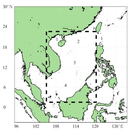
Fig.1.The study areas over the SCS.1：Beibu Gulf；2：northern SCS；3：middle SCS；and 4：southern SCS.

2.2 Methodology

The new evaporation duct climatology is computed from a series of procedures（Fig.2）.Firstly，the atmospheric data used to calculate the EDH are obtained from the NCEP CFSR and the reliability of the data is verified by using weather buoy observations from the Pacific Ocean.Secondly，the EDHs are calculated in the study area by using an improved evaporation duct model.Thirdly，a comparison between the EDH of the new and old climatologies is presented. Finally，the spatiotemporal characteristics of the evaporation duct over the SCS are analyzed.

2.2.1 An improved evaporation duct model

The EDH is usually determined by using an evaporation duct model.In recent years，a number of evaporation duct models such as the PJ model（Paulus，1985），the Musson-Gauthier-Bruth（MGB）model（Musson et al.，1992），the Liu-Katsaros-Businger（LKB）model（Liu et al.，1979；Babin and Dockery，2002），the Babin-Young-Carton（BYC）mod-el（Babin et al.，1997），and the Navy Atmospheric Vertical Surface Layer（NAVSLaM）model（Frederickson et al.，2000；Frederickson，2012）have been developed to calculate EDHs.The NAVSLaM model was previously（before 2012）called the Naval Postgraduate School（NPS）model.Babin et al.（1997）and Babin and Dockery（2002）tested the PJ，NAVSLaM，BYC，MGB，and NRL models carefully using ocean buoy data；they summarized that the NAVSLaM model was the optimal model for estimating the modified refractivity profile.However，they believed that the NAVSLaM model still overestimated the EDH，especially in very strong and stable conditions.Then，Frederickson（2012）used new stability functions to improve the NAVSLaM model's performance in stable conditions. The NAVSLaM model uses the Beljaar and Holtslag'sstability function （Frederickson etal.，2000）in stable conditions（air-sea temperature difference（ASTD）＞0℃），hereafter referred to as the NAVSLaM-BH model.The Beljjar and Holtslag's function has been proven to be suitable only for weak stable conditions and leads to very high EDHs under some stable conditions（Frederickson，2012）.Cheng's stability function（Cheng and Brutseaert，2005）and Grachev's stability function（Grachev et al.，2007）are obtained from recent boundary layer experiments. These functions perform better（Frederickson，2012）in stable conditions with the NAVSLaM model（hereafter referred to as the NAVSLaM-CB and NAVSLaM-GR models，respectively）.

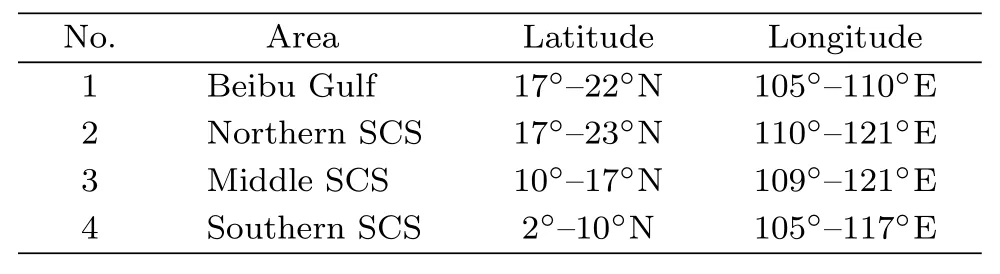
Table 1.The domains of the areas under study

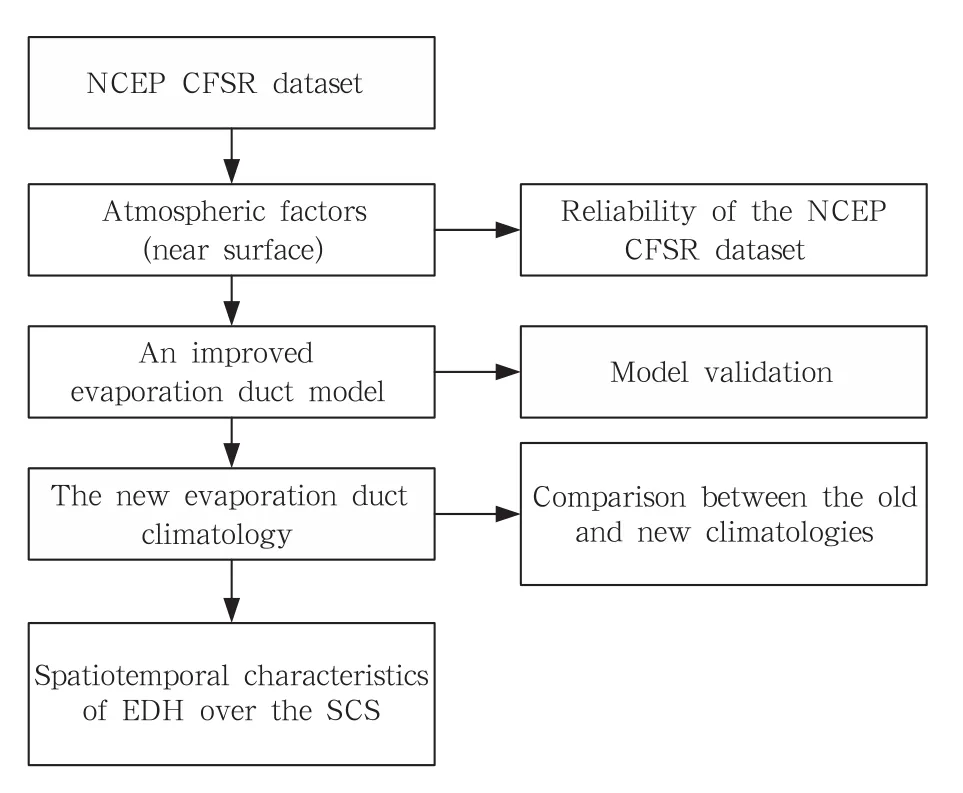
Fig.2.Flow chart showing the procedures used in this study to calculate and analyze EDH.

In this study，the modified refractivity profiles calculated by using different stability functions，with air temperature of 20℃，ASTD of 2℃，relative humidity of 72%，wind speed of 5.3 m s-1，and pressure of 1022.2 hPa，show that the NAVSLaM-BH model cannot define the EDH under these stable conditions（green line in Fig.3a）.The NAVSLaM-CB model defines the EDH as 70.5 m（blue line in Fig.3a）and the NAVSLaM-GR model defines the EDH as 54.9 m（red line in Fig.3a）.

The EDH sensitivity analyses performed by using the three model configurations，with air temperature of 25℃，ASTD of 0-6℃，relative humidity of 50%-90%，wind speed of 3 m s-1，and pressure of 1000 hPa，show that the EDH increases quickly as the ASTD increases（Figs.3b-d）.The EDH also decreases as the relative humidity increases.Under stable conditions，the temperature inversion is the primary cause of the high EDH.The NAVSLaM-BH model cannot define the EDH when the ASTD is greater than 2℃（Fig.3b）under low relative humidity conditions.Meanwhile，the NAVSLaM-CB（Fig. 3c）and NAVSLaM-GR（Fig.3d）models have much wider regions of applicability under stable conditions，especially the NAVSLaM-GR model.

Frederickson（2012）validated the NAVSLaM model using measurements collected during the experiment over Wallops Island，VA in 2000. Frederickson（2012）input the modified refractivity profiles computed by the NAVSLaM model into the Advanced Propagation Model（APM；Barrios and Patterson，2002）to calculate the propagation loss.The results showed that the NAVSLaM-GR model simulation agreed best with the propagation measurements. Therefore，the NAVSLaM-GR model configuration is chosen to compute the EDH in this paper.

2.2.2 NCEP CFSR dataset

The NCEP CFSR dataset provides effective data to investigate the spatiotemporal characteristics of evaporation ducts.The NCEP and NCAR have collaborated（and continue to do so）on this reanalysis project，to produce the record of global atmospheric fields，and support the research and climate monitor-ing communities. Their efforts involve the recovery of observational data from land，surface，ship，radiosonde，aircraft，and satellite instruments；then，quality control procedures are performed and the data are assimilated by using a data assimilation system that is kept unchanged over the specified reanalysis period.

Fig.3.（a）Modified refractivity profiles computed by using the three different NAVSLaM model configurations.（b-d）EDH values derived from the（b）NAVSLaM-BH，（c）NAVSLaM-CB，and（d）NAVSLaM-GR model configurations.

The NCEP CFSR product for the 31-yr period

（1979-2009）was completed in January 2010.The CFSR was designed and executed as a global，high resolution，coupled atmosphere-ocean-land surface-sea ice system，to provide the best estimate of the state of these coupled domains over the specified period（Saha et al.，2010）.One-hour reanalysis data are available from 1979 to the present day and global atmospheric fields are provided for a variety of atmospheric variables.The spatial coverage comprises 1152×576 grid points over 89.761°N-89.761°S，180°W-180°E，which provide data with a high horizontal resolution（0.313°×0.312°）.The old evaporation duct climatology was computed from the ICOADS during 1974-1980 and used Marsden squares，with a spatial resolution of 10°×10°.The atmospheric variables obtained directly from the NCEP CFSR dataset and those calculated from the available data are shown in Table 2.

Thelong-term NationalData Buoy Center（NDBC）data are used to confirm the reliability of the NCEP CFSR data.Buoy data are considered the best available as a comparison benchmark，because the measurements are not affected by the land or research vessel（Newton，2003）.

The tropical atmosphere ocean（TAO）array is in the tropical Pacific Ocean and telemeters oceanographic and meteorological data to shore in real-time.

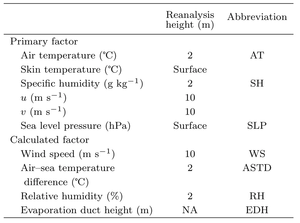
Table 2.Primary atmospheric variables obtained from the NCEP CFSR and those calculated from the available data

The buoy WMO52006， located at 8°2′54′′N，165°8′31′′E，was selected to confirm the reliability of the NCEP CFSR data.The data from 16 July 1989 to 31 December 2009 were processed.Twenty years of monthly mean values were obtained by averaging the appropriate daily values of each month.

The meteorological variables obtained by the buoy and the NCEP CFSR dataset during 1-30 April 2009 show that，in general，the NCEP CFSR data agree well with the buoy measurement data（Fig.4a）. However，the NCEP CFSR data do deviate slightly from the buoy data at some points in April 2009；these deviations may be caused by data assimilation techniques and the lack of observational data.

The monthly average（Fig. 4b）and standard deviation（Fig. 4c）of the meteorological variables derived from the NCEP CFSR dataset are consistent with the buoy data.The monthly averages of the derived EDHs also show good agreement between the NCEP CFSR and the buoy data，with the maximum difference of about 1 m （Fig.4d）.From January to March，the EDH calculated from the buoy data is higher than that obtained from the NCEP CFSR dataset，because the air temperature is higher and the relative humidity is lower，according to the buoy data.The maximum difference between the monthly standard deviations of EDH is less than 0.5 m（Fig. 4e）；the uncertainty of the EDH due to deviations in the NCEP CFSR data from the buoy observations is discussed in the Appendix.Overall，these comparisons show that the NCEP CFSR dataset is reliable for constructing the EDH climatology over the SCS.

In this paper，the reference height of atmospheric variables is set to 2 m in the NAVSLaM-GR model（the same height as that used for air temperature and relative humidity）.The reanalysis height of wind speed from the NCEP CFSR data is 10 m.However，as shown in Fig.4a，the NCEP CFSR data are consistent with the wind speed data from the buoy（with measurement height of about 2 m）.Thus，the NCEP CFSR wind speed data are used in the evaporation duct model.

2.2.3 The APM propagation model

The parabolic equation（PE）method has been widely used to calculate electromagnetic wave propagation in evaporation ducts.The advantage of the PE method is that it can simulate electromagnetic wave propagation in a range-dependent troposphere environment.The standard parabolic equation can be obtained from the Helmholtz equation，with certain assumptions，and expressed in the form of

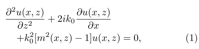
where u represents a scalar component of the electric field for horizontal polarization，or a scalar component of the magnetic field for vertical polarization，z is the height，x is the range，k0is the free space wave number，and m is the modified refractive index.

In this paper，the APM is used to calculate the electromagnetic wave propagation in the evaporation duct（Space and Naval Warfare Systems Center，2006；Barrios and Patterson，2002）.The APM model is a hybrid model that combines the radio physical optics（RPO）model and terrain parabolic equation model（TPEM）in a relatively fast code.The APM is used in the AREPS，which is used widely for the assessment of electromagnetic systems.The APM has also been validated in various terrain and evaporation duct environments（Anderson et al.，2004；Barrios et al.，2006）.

3.Results

The spatiotemporal characteristics of the EDHduring different months in the SCS are inhomogeneous（Fig.5；Table 3）.The characteristics for the different areas in the SCS are analyzed below.

Fig.4.Comparison between the NDBC buoy observations and the NCEP CFSR data at the nearest grid point.（a）Air temperature（AT），sea surface temperature（SST），wind speed（WS），and relative humidity（RH）during 1-30 April 2009；（b）monthly mean values and（c）standard deviations of these variables（squares：buoy data；circles：NCEP CFSR data）；and（d）monthly mean values and（e）standard deviations of the EDH.

（1）The Beibu Gulf：the average EDH is low in January and February（＜10 m）and high in April，May，and July；it is highest in July（average 13.8 m）. In summer，the maximal height of the EDH（＞20 m）appears in the northwest of Hainan Island and thenortheast of Vietnam.The EDH decreases a little in autumn，but in November，as winter approaches，the whole area has a high EDH.The standard deviation of the EDH in the Beibu Gulf is higher than in other parts of the SCS，reaching a maximum in April（4.5 m）.

Fig.5.Spatiotemporal characteristics of the EDH（m）over the SCS.（a）-（l）January-December.

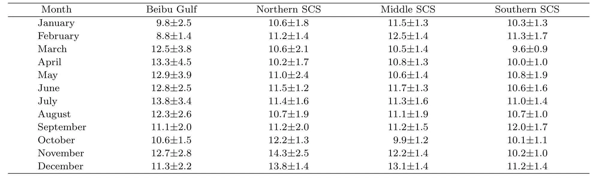
Table 3.Statistics of the EDH（m）in different regions of the SCS（mean±standard deviation；m）

（2）The northern SCS：during January-August，the average EDH ranges between 10 and 12 m.The average EDH increases rapidly during September-November，when it reaches its maximum value（average 14.3 m）.Then，from December to next February，the EDH quickly decreases to about 10 m；the minimum average EDH occurs in April（10.2 m）.The maximal EDH always appears between the Taiwan Region and the Philippines during spring-，summer-，and wintertime.In November and December，the EDH is high across the whole area.The standard deviation of the EDH is highest in November（2.5 m）.

（3）The middle SCS：the maximum and minimum average EDHs occur in December（13.1 m）and October（9.9 m），respectively.During wintertime，the whole area has a high EDH.As spring approaches，there is an obvious decrease of the EDH and the minimal EDH occurs in the south of the area.In summertime，the EDH remains above 10 m and the maximal band moves to the southeast of Vietnam；this region is far from the coast.The standard deviation of the EDH is relatively stable throughout the year（＜2 m）.

（4）The southern SCS：the maximum and minimum EDHs occur in September（12.0 m）and March（9.6 m），respectively.During wintertime，the minimal EDH（＜10 m）occurs in the northwest of Malaysia.As spring approaches，the EDH increases rapidly and the maximal height appears in the southern part of this area in May.During September-October，the EDH quickly decreases to around 10 m.The standard deviation of the EDH is relatively stable in this region（＜2 m）.

4.Discussion

4.1 Comparison of EDHs derived from the old and new climatologies

Comparison between the monthly average EDHs of the old and new climatologies in the SCS reveals differences in their magnitudes（Fig.6）.The old climatology overestimates the monthly average EDH，which is between 15 and 18 m（Fig.6a）.The monthly average EDH is between 10 and 12 m throughout the year in the new climatology；the monthly average reaches maximum in December（12.2 m）and minimum in March（10.4 m）.The standard deviation of the EDH for the new climatology is also relatively stable（＜1.5 m；Fig.6b）.

A spatial comparison of the EDH between the old and new climatologies in December shows that the new climatology has a better spatial resolution of the EDH in the SCS（old：10°×10°；new：0.312°×0.313°；Figs.6c and 6d）.A comparison of the statistical features of the EDH near Huangyan Island in December shows that the monthly average EDH in the old climatology is 17.95 m，but it is 12.42 m in the new one. The monthly average EDH and the standard deviation are overestimated in the old climatology.This overestimation causes significant impacts on the modeling of electromagnetic wave propagation in evapora-tion ducts.

The APM （Barrios and Patterson，2002；Space and Naval Warfare Systems Center，2006）and the monthly average EDH in Huangyan Island are used here to model the electromagnetic wave propagation in the evaporation duct.The modified refractivityprofiles show that the EDHs of the old and new climatologies are 17.95 and 12.42 m，respectively（Fig. 7a）.The modified refractivity profiles are input into the APM model to calculate path loss；in the simulation，the transmitting antenna height is 10 m，the electromagnetic wave frequency is 10 GHz，the polarization of the electromagnetic waves is horizontal，the antenna pattern is omnidirectional，and the computed distance is 100 km.

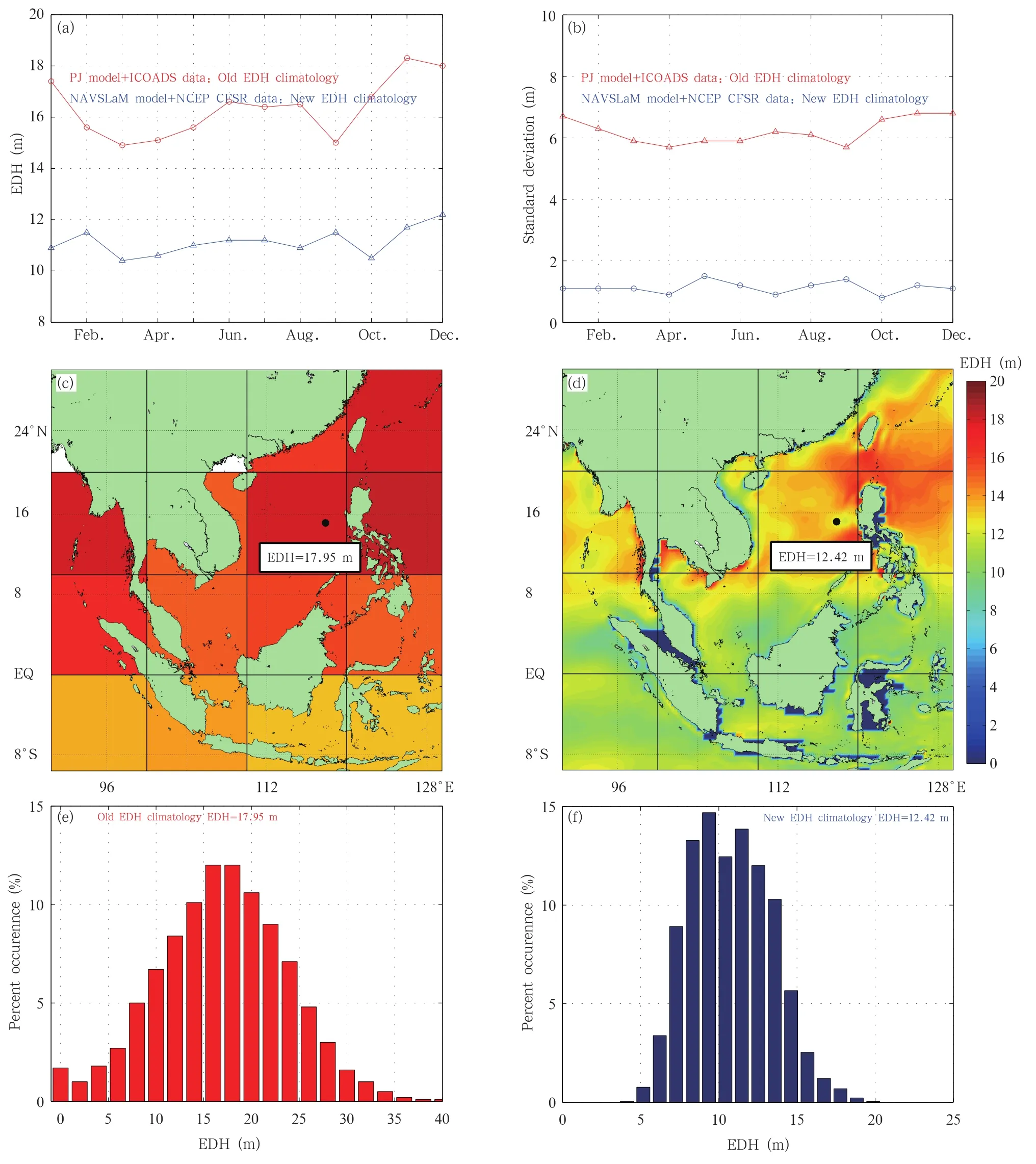
Fig.6.Comparison between the（a）monthly average and（b）standard deviation of the EDHs in the old and new climatologies over the SCS.（c，d）Spatial variations of the EDH in December and（e，f）statistical features of the EDH near Huangyan Island in December，based on the（c，e）old and（d，f）new climatologies.

The path loss computed by the APM shows that when the EDH is 17.95 m，the path loss at 10 m is less than that calculated when the EDH is 12.42 m（Figs.7b and 7c）.The path loss simulated at 100 km with the new climatology is 145 dB，while it is 137 dB（height：10 m）with the old climatology.Thus，the new climatology results in about an 8-dB increase at the range of 100 km.This difference will cause significant impacts on the predictions of the radar detection and communication ranges.

4.2 Spatiotemporal characteristics of the EDH over the South China Sea

Sensitivity analyses of the meteorological parameters revealed a couple of important features（Fig. 8）.Firstly，under unstable conditions（ASTD＜0℃），there is a stronger evaporation duct，with higher air and sea surface temperatures，higher wind speed，and lower relative humidity.Secondly，under stable conditions（ASTD＞0℃），the ASTD affects the EDH significantly，and the relationships between the EDHand the meteorological parameters are more complicated.A very high evaporation duct will occur with higher air and sea surface temperatures，lower wind speed，and lower relative humidity.

Fig.7.Comparison of the EDH effect of the old and new climatologies on electromagnetic wave propagation in the evaporation duct.（a）The modified refractivity profile（red line：old climatology；blue line：new climatology），（b）the path loss at the height of 10 m，and the path loss（shading；dB）distributions of（c）old and（d）new EDH climatologies.

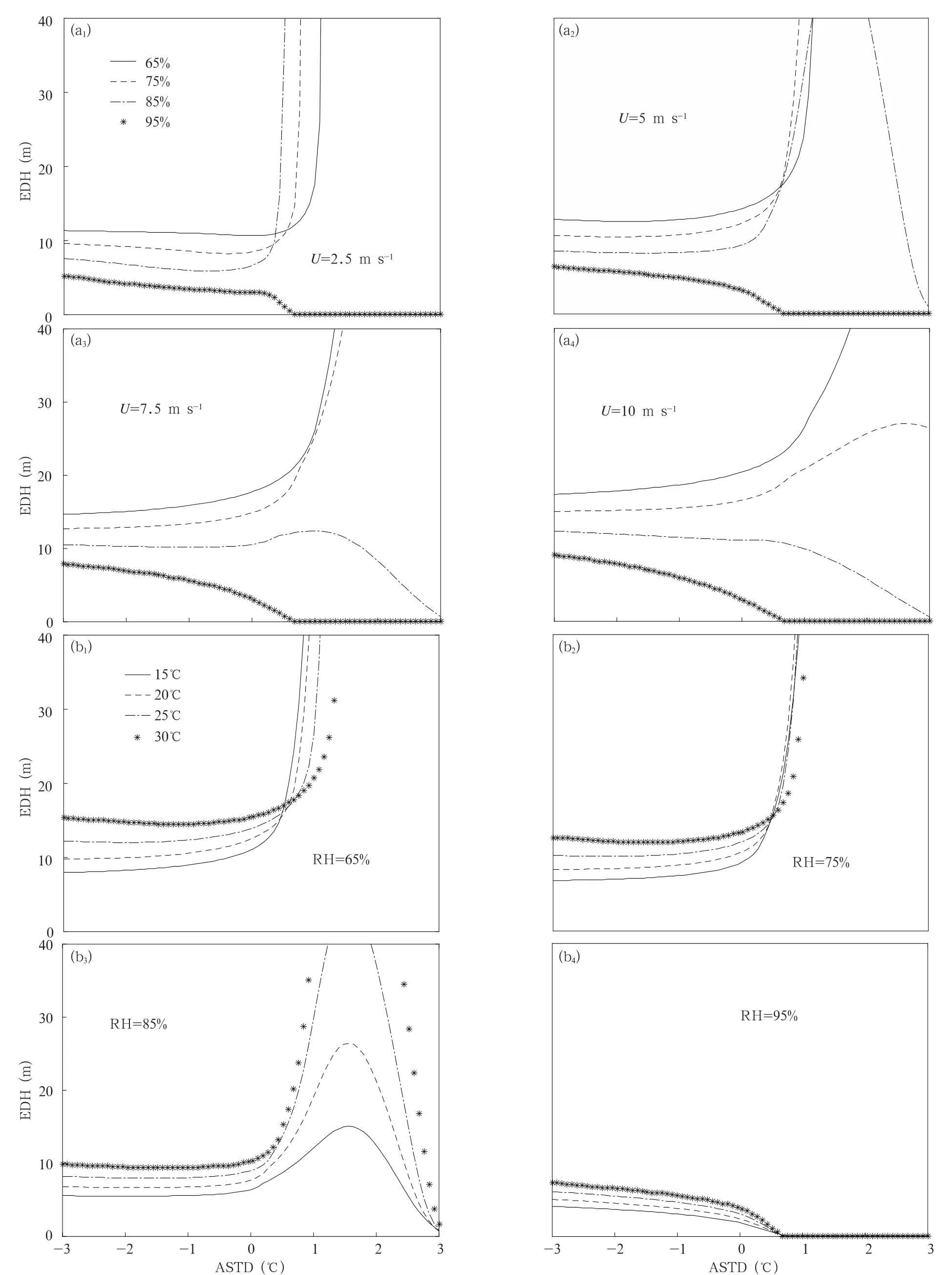
Fig.8.Sensitivity analyses of the EDH computed by using the evaporation duct model when（a1-a4）sea surface temperature is 26℃and（b1-b4）wind speed is 5 m s-1.

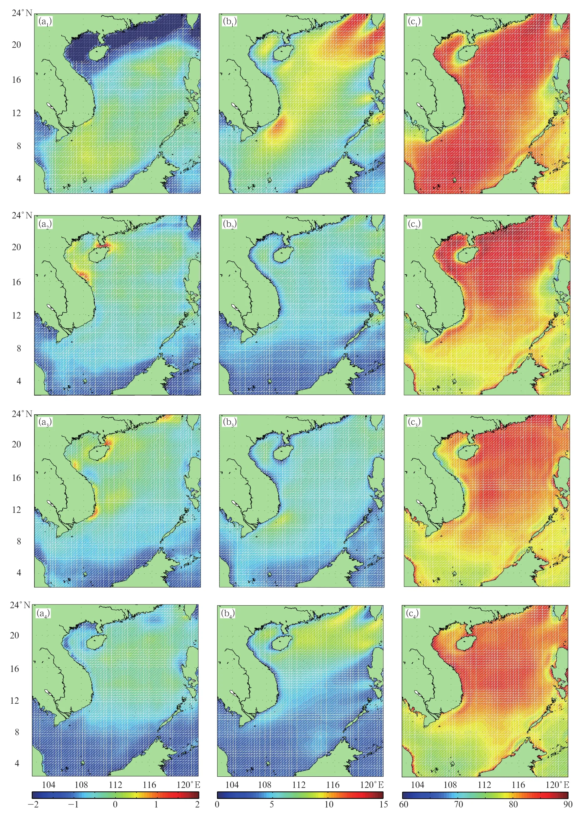
Fig.9.Spatiotemporal characteristics of（a1-a4）ASTD（℃），（b1-b4）wind speed（m s-1），and（c1-c4）relative humidity（%）over the SCS for（a1，b1，c1）January，（a2，b2，c2）April，（a3，b3，c3）July，and（a4，b4，c4）October.

The spatiotemporal characteristics of the ASTD，wind speed，and relative humidity over the SCS during different months（Fig.9）reveal the causes of the spatiotemporal characteristics of the EDH in the different regions，as discussed below.

（1）The Beibu Gulf：the EDH is high from October to November，and during this period the ASTD is negative，resulting in unstable conditions（Fig.9a）. The high wind speeds（more than 10 m s-1；Fig. 9b）and low relative humidity（less than 70%；Fig. 9c）cause the high EDH in this area during October-November.

（2）The northern SCS：the EDH is very high in winter，during which there are unstable conditions in this area（ASTD＜-2℃；Fig.9a）.The wind speeds are more than 12 m s-1and the relative humidity is less than 75%during winter（Figs.9b and 9c），which increases the EDH.In June and July，there are neutral or stable conditions in the area，and the high relative humidity makes the EDH low（Fig.9c）.

（3）The middle SCS：in this area，there are neutral or unstable conditions throughout the year.The EDH is between 10 and 12 m in most months，and the relative humidity is above 80%in this area.The wind speeds are more than 10 m from November to next February，which causes relatively high EDHs during this period.

（4）The southern SCS：the EDH is about 10 m from April to November.During this period，there are unstable conditions in the area（ASTD＜0℃）. The wind speeds are less than 5 m s-1and the relative humidity is above 75%；the low wind speeds are the primary cause of the low EDH in this area.In March，stable conditions prevail，and the high relative humidity and low sea surface temperature make the EDH low.

5.Conclusions

This paper presents a new evaporation duct climatology over the SCS.The primary work of this paper is summarized as follows：

（1）The new evaporation duct climatology is computed by using a state-of-the-art evaporation duct model（the NAVSLaM-GR model）and an improved meteorology dataset（NCEP CFSR dataset）. The new climatology provides a better spatial resolution（0.312°×0.313°）of the EDH over the SCS.

（2）The spatiotemporal characteristics of the evaporation duct over the SCS are analyzed based on the new climatology.Generally speaking，the EDH is higher in winter than in other seasons.The spatiotemporal characteristics for each part of the SCS are discussed.

（3）A comparison between the EDH of the new and old climatologies is performed.In the new climatology，the monthly average EDH is between 10 and 12 m，and the standard deviation of the EDH is below 1.5 m over the SCS；the corresponding values derived from the old climatology are overestimated.

（4）A comparison between the statistical features of the EDH near Huangyan Island in the new and old climatologies is also presented.The differences and their impacts on electromagnetic wave propagation are discussed.

The characteristics of the new evaporation duct climatology make it possible to investigate the effects of the horizontally inhomogeneous evaporation duct on electromagnetic wave propagation.It will be valuable to study shipborne electromagnetic systems'performances，based on the statistical characteristics of the evaporation duct over the SCS.

APPENDIX

The uncertainty of the EDH is estimated based on the NCEP CFSR data and the buoy data（in Section 2.2.2）in 2008.The EDH derived from the NCEP CFSR data（NCEP EDH）and the EDH derived from the the buoy data（buoy EDH）in 2008 show that，in general，the EDHs derived from the two datasets are consistent（Figs.A1a and A1b），although there are some differences between the NCEP EDH and the buoy EDH.The average and standard deviation of the differences in the EDH are 1.08 and 1.64 m，respectively.The probability distribution of the differences in the EDH in 2008（between the two datasets）showsthat the probability that the differences in the EDH ranged from-2 to 2 m is near 80%for 2008（Fig.A1c）.

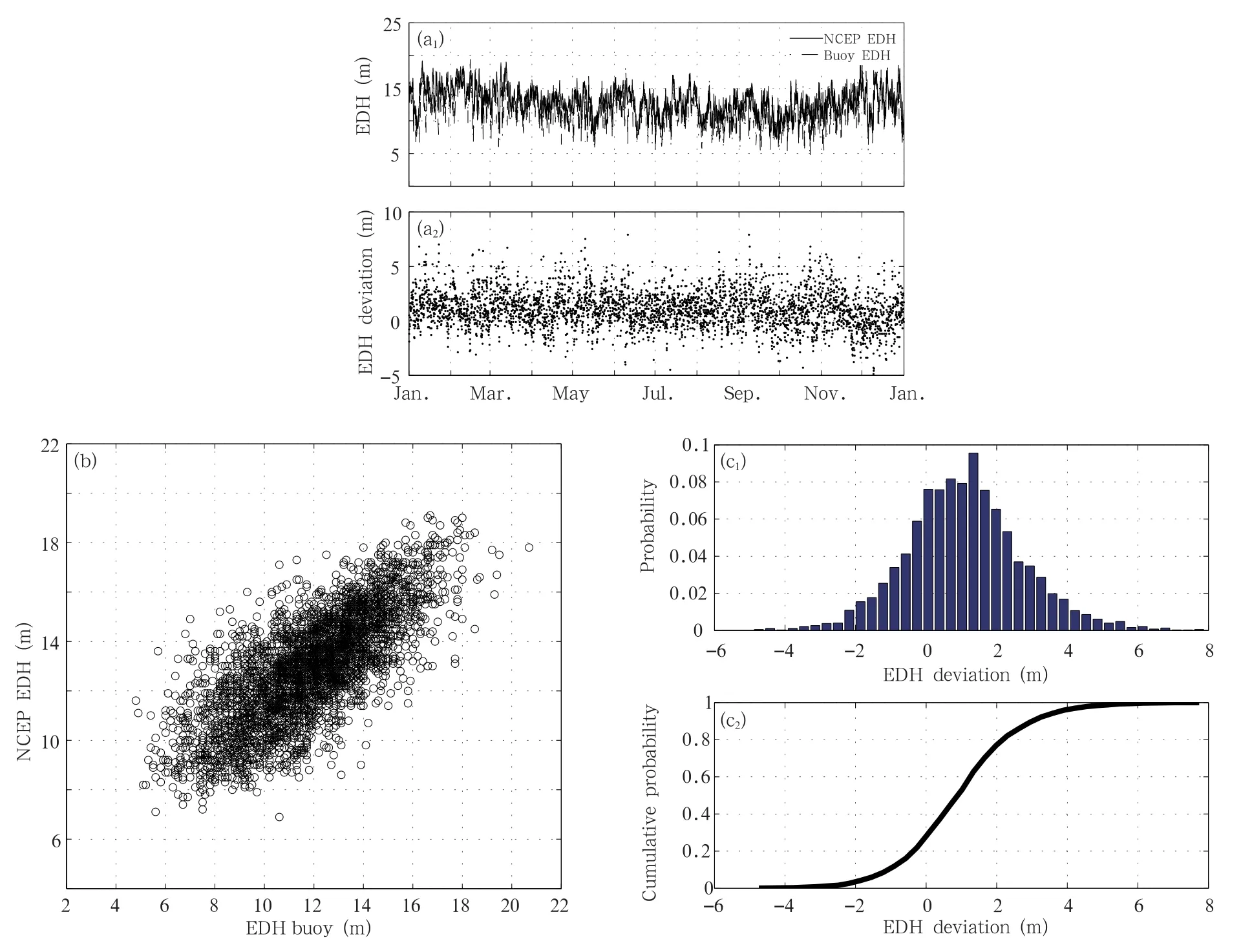
Fig.A1.The uncertainty of the EDH，analyzed by the differences between the EDHs derived from the NCEP CFSR data and the buoy observational data.（a1）Comparison between the buoy EDH and NCEP EDH，（a2）EDH deviation，（b）comparison between the NCEP EDH and the buoy EDH，（c1）inpterval probability of the EDH difference，and（c2）accumulation probability of the EDH difference.

Acknowledgments.We would like to thank Lei Bo，Yan Xidang，and Zhang Qi at Northwestern Polytechnical University for their helpful discussion on this paper.

Anderson，K.D.，1995：Radar detection of low-altitude targets in a maritime environment.IEEE Trans. Antennas Propag.，43，609-613.

Anderson，K.D.，S.Doss-Hammel，D.Tsintikidis，et al.，2004：The RED experiment：An assessment of boundary layer effects in a trade winds regime on microwave and infrared propagation over the sea. Bull.Amer.Meteor.Soc.，85，1355-1365.

Babin，S.M.，G.S.Young，and J.A.Carton，1997：A new model of the oceanic evaporation duct.J.Appl. Meteor.，36，193-204.

Babin，S.M.，and G.D.Dockery，2002：LKB-based evaporation duct model comparison with buoy data.J. Appl.Meteor.，41，434-446.

Barrios，A.E.，and W.L.Patterson，2002：Advanced propagation model（APM）ver.1.3.1 computer software configuration item（CSCI）documents，1-10.

Barrios，A.E.，K.D.Anderson，and G.Lindem，2006：Low altitude propagation effects—A validation study of the advanced propagation model（APM）for mobile radio applications.IEEE Trans.Antennas Propag.，54，2869-2877.

Cheng，Y.G.，and W.Brutseaert，2005：Flux-profile relationships for wind speed and temperature in the stable atmospheric boundary layer.Bound.-Layer Meteor.，114，519-538.

Cheng Yinhe，Zhou Shengqi，and Wang Dongxiao，2013a：Review of the study of atmospheric ducts over the sea.Adv.Earth Sci.，28，318-326.（in Chinese）

Cheng Yinhe，Zhang Yusheng，Zhao Zhenwei，et al.，2013b：Analysis on the evaporation duct environment near coast of the northern South China Sea in winter.Chinese J.Radio Sci.，28，697-703.（in Chinese）

Ding Juli，Fei Jianfang，Huang Xiaogang，et al.，2015a：Development and validation of an evaporation duct model.Part I：Model establishment and sensitivity experiments.J.Meteor.Res.，29，467-481.

Ding Juli，Fei Jianfang，Huang Xiaogang，et al.，2015b：Development and validation of an evaporation duct model.Part II：Evaluation and improvement of stability functions.J.Meteor.Res.，29，482-495.

Frederickson，P.A.，2012：Improving the Characterization of the Environment for AREPS Electromagnetic Performance Predictions.Weather Impacts Decision Aids（WIDA）Workshop.Reno，NV，6-8.

Frederickson，P.A.，K.L.Davidson，and A.K.Goroch，2000：Operational evaporation duct model for MORIAH.Naval Postgraduate School Report，10-25.

Grachev，A.A.，E.L.Andreas，C.W.Fairall，et al.，2007：SHEBA flux-profile relationships in the stable atmospheric boundary layer.Bound.-Layer Meteor.，124，315-333.

Hitney，H.V.，and L.R.Hitney，1990：Frequency diversity effects of evaporation duct propagation.IEEE Trans.Antennas Propag.，38，1694-1700.

Jiao Lin and Zhang Yonggang，2009：An evaporation duct prediction model coupled with the MM5.Acta Meteor.Sinica，67，382-387.（in Chinese）

Levy，M.F.，and K.H.Craig，1989：Case studies of transhorizon propagation：Reliability of predictions using radiosonde data.Sixth International Conference on Antennas and Propagation.IEEE，Coventry，456-460.

Li Yunbo，Zhang Yonggang，Tang Haichuan，et al.，2009：Oceanic evaporation duct diagnosis model based on air-sea flux algorithm.J.Appl.Meteor.Sci.，20，628-633.（in Chinese）

Liu，W.T.，K.B.Katsaros，and J.A.Businger，1979：Bulk parameterization of air-sea exchanges of heat and water vapor including the molecular constraints at the interface.J.Atmos.Sci.，36，1722-1735.

Musson-Genon，G.L.，S.Gauthier，and E.Bruth，1992：A simple method to determine evaporation duct height in the sea surface boundary layer. Radio Sci.，27，635-644.

Newton，D.A.，2003：COAMPS modeled surface layer refractivity in the roughness and evaporation duct experiment 2001.Naval Postgraduate Dissertation，23 pp.

Paulus，P.A.，1985：Practical application of an evaporation duct model.Radio Sci.，20，887-896.

Pons，J.，S.C.Reising，S.Padmanabhan，et al.，2003：Passive polarimetric remote sensing of the ocean surface during the Rough Evaporation Duct experiment（RED 2001）.2003 IEEE International Geoscience and Remote Sensing Symposium.IEEE，Toulouse，2732-2734.

Saha，S.，S.Moorthi，H.L.Pan，et al.，2010：The NCEP climate forecast system reanalysis. Bull. Amer. Meteor.Soc.，91，1015-1057.

Space and Naval Warfare Systems Center，2006：User's manual（UM）for Advanced Refractive Effects Prediction System Version 3.6，285 pp.

Twigg，K.L.，2007：A smart climatology of evaporation duct height and surface radar propagation in the Indian Ocean.Ph.D.dissertation，Naval Postgraduate School，26 pp.

Wash，C.H.，and K.L.Davidson，1994：Remote measurements and coastal atmospheric refraction.Geoscience and Remote Sensing Symposium. IEEE，Pasadena，397-401.

Woods，G.S.，A.Ruxton，C.Huddlestone-Holmes，et al.，2009：High-capacity，long-range，over ocean microwave link using the evaporation duct.IEEE J. Oceanic Eng.，34，323-330.

Yao Zhanyu，Zhao Bolin，Li Wanbiao，et al.，2000：The analysis on charateristics of atmospheric duct and its effects on the propagation of eletromagnetic wave. Acta Meteor.Sinica，58，605-616.（in Chinese）

Yardim，C.，P.Gerstoft，and W.S.Hodgkiss，2008：Tracking refractivity from clutter using Kalman and particle filters.IEEE Trans.Antennas Propag.，56，1058-1070.

Zhao Xiaofeng，Wang Dongxiao，Huang Sixun，et al.，2013：Statistical estimations of atmospheric duct over the South China Sea and the tropical eastern Indian Ocean.Chin.Sci.Bull.，58，2794-2797.

Shi Yang， Yang Kunde， Yang Yixin， et al.， 2015： A new evaporation duct climatology over the South China Sea. J. Meteor. Res.， 29（5）， 764-778，

10.1007/s13351-015-4127-6.

（Received December 11，2014；in final form June 30，2015）