
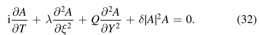
Modulation instability analysis of Rossby waves based on (2+1)-dimensional highorder Schrödinger equation
2022-08-02 03:01CongWang王丛JingjingLi李晶晶andHongweiYang杨红卫
关键词:晶晶
Cong Wang (王丛), Jingjing Li (李晶晶) and Hongwei Yang (杨红卫)
College of Mathematics and Systems Science, Shandong University of Science and Technology, Qingdao 266590, China
Abstract Modulational instability is an important area of research with important practical and theoretical significance in fluid mechanics, optics, plasma physics, and military and communication engineering.In this paper, using multiscale analysis and a perturbation expansion method,starting from the quasi-geostrophic potential vortex equation, a new (2+1)-dimensional highorder nonlinear Schrödinger equation describing Rossby waves in stratified fluids is obtained.Based on this equation, conditions for the occurrence of modulational instability of Rossby waves are analyzed.Moreover, the effects of factors such as the dimension and order of the equation and the latitude at which Rossby waves occur on modulational instability are discussed.It is found that the(2+1)-dimensional equation provides a good description of the modulational instability of Rossby waves on a plane.The high-order terms affect the modulational instability,and it is found that instability is more likely to occur at high latitudes.
Keywords: (2+1)-dimensional high-order nonlinear Schrödinger equation, modulation instability, Rossby waves, stratified fluids
1.Introduction
Among the most important types of waves that arise in geophysical fluid dynamics are Rossby waves:long waves with a large horizontal scale and a long life cycle that occur in both the atmosphere and ocean.These waves have quasi-horizontal and non-amplitude dispersive characteristics.In the atmosphere, they propagate at the wind speed, i.e.much more slowly than sound waves and gravity waves.The horizontal scale of Rossby waves is of the order of the radius of the Earth,and so they are also called large-scale planetary waves[1–3].Rossby waves have significant effects on large-scale weather processes and are responsible for a wide range of oceanic and atmospheric phenomena, such as the North Atlantic Oscillation, the eddy forming the Gulf of Mexico oceanic current, and the blocking that occurs high in the atmosphere[4,5].Not only are Rossby waves involved in the formation of ocean currents, but at the same time, ocean currents will create new Rossby waves, as is the case for the Kuroshio and the Eastern Australia Current [6–8].The interannual characteristic behavior of the ocean is also affected by Rossby waves, as in the case of the El Niño phenomenon [9].Therefore, Rossby waves are of great significance in oceanography and meteorology and have become an increasingly important research topic in hydrodynamics.
Over the years, a wide variety of equations have been applied to the study of Rossby waves in the atmosphere and ocean.Long first studied Rossby waves in positive-pressure fluids in 1964 and obtained a description of the changes in their amplitude in terms of the Korteweg–de Vries (KdV)equation, thereby laying an important foundation for further study of these waves [10].Then, in 1966, Benney obtained important conclusions about the velocity and amplitude of Rossby waves [11].Using a stratified fluid model, Wadati derived a modified KdV (mKdV) equation describing the amplitude of Rossby waves [12].Lou derived the coupled KDV equations describing Rossby waves in two layers of fluid [13].Number of other types of equations have been proposed to describe Rossby waves, including, for example,the Boussinesq equation, the Zakharov–Kuznetsov (ZK)equation, and the nonlinear Schrödinger (NLS) equation,among which the NLS equation has been particularly widely used [14].
Benney and Yamagata were the first to propose that atmospheric Rossby waves could be described by the NLS equation [15, 16].Equations describing the evolution of Rossby waves usually contain nonlinear high-order terms In previous studies,high-order terms had normally been ignored.However, when the parameters associated with high-order terms are sufficiently large, the effects of these terms cannot be ignored.Therefore, interest arose in the use of high-order nonlinear Schrödinger (HNLS) equations to describe Rossby waves.Although attention initial focused on (1+1)-dimensional equations, the development of appropriate mathematical tools allowed the use of (2+1)-dimensional equations for Rossby waves in two-dimensional space[17].Luo studied an HNLS equation to describe changes in the amplitude of Rossby waves in the ocean and atmosphere [18].On this basis, Huang continued to study such high-order NLS equations [19].
Modulational instability occurs widely in various nonlinear media and can be observed in many fields,such as fluid mechanics [20], plasma physics [21], and optics [22].Modulational instability refers mainly to the unstable situation that occurs during the propagation of steady-state waves owing to the influence of dispersion and nonlinear effects.It is a nonlinear process in which a plane wave passes through a nondispersive medium, generating amplitude and frequency self-modulation, as a result of which a tiny disturbance superimposed on the plane wave will grow exponentially[23, 24].Modulational instability can be invoked to provide understanding to the generation mechanism of rogue waves and breather solutions, and also can study resonance excitation in a modulationally unstable region and baseband modulational instability [25–27].In previous studies, many scholars used high-order NLS equations to analyze modulation instability.Lu et al have provided a method to analyze modulational instability based on a third-order NLS equation[28].Yue studied the modulational instability and rogue waves of the sixth-order nonlinear Schrödinger equation[29].Study of the modulational instability of Rossby waves can enable more accurate prediction of their propagation,which is of great significance for physical oceanography, atmospheric physics, military and communication engineering, etc.There have been extensive investigations of the modulational instability of Rossby waves,and the methods used have been extended to other nonlinear waves,such as gravity waves and internal solitary waves [30–32].
In this paper,a new(2+1)-dimensional high-order NLS equation describing Rossby waves is derived in the context of stratified fluids.On this basis,the modulational instability and propagation characteristics of Rossby waves are studied.The remainder of the paper is organized as follows.In section 2,a dimensionless form of quasi-geostrophic potential vortex equation in stratified fluids is presented, and a (2+1)-dimensional high-order NLS equation describing Rossby waves is obtained through a multi-scale analysis and an iterative perturbation method [33].In section 3, based on the newly derived equation, the conditions that produce modulational instability are analyzed.In section 4, the effect of factors such as the dimension and order of the equation and the latitude of Rossby waves on modulational instability are discussed, and changes in the modulational instability gain and region are described.Conclusions are given in section 5.
2.Derivation of (2+1)-dimensional high-order NLS equation
We consider the quasi-geostrophic vorticity equation without any external force,topography,or frictional dissipation under the β effect.We suppose that the β effect is a nonlinear function of y andφ is the total flow function.N is the Väisälä frequency used to measure the stability of the stratified fluid.Then, the equation takes the form
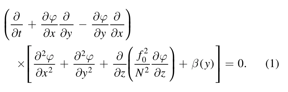
We define dimensionless variables (indicated by primes ′) as follows:
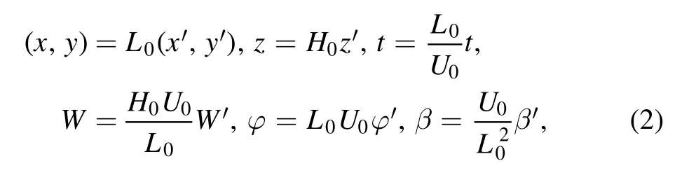
where L0is a characteristic horizontal length scale, H0is a characteristic fluid thickness, and U0is a characteristic fluid velocity.When these variables are used in equation (1), it takes the following dimensionless form(with the primes now omitted from the dimensionless variables):

Here,
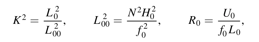
L00is usually called deformation radius andf0= 2Ω sinθis called the Coriolis parameter,where Ω is the angular velocity of the Earth.
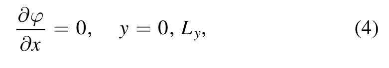
The flow is confined within the boundary of the β effect,which is characterized by a width Ly, and so
while the zonal average flow function(y,t)satisfies

We assume that the basic zonal flow is Ψ(y)=∫(−u)dy, and so the total flow function satisfies
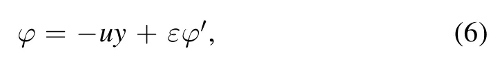
where u is an undetermined constant, representing the wave velocity of the nondispersive part of the linear Rossby wave.ε is a small parameter,which is related to the amplitude of the perturbation wave assumed to be finite.Andφ′ is the disturbance flow function.Substituting equation (6) into equation (3), and omitting the prime on the perturbed stream functionφ′, we obtain
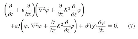
whereβ′ is the first derivative of β(y),

and
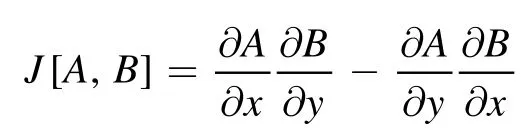
is the Jacobian determinant.
Atmospheric dynamics involves motion on two time scales, associated with rapid and slow changes, respectively.We introduce the following slow stretch coordinates:

where ε is a small parameter and Cgis the group velocity of Rossby waves.We then have the following transformations:
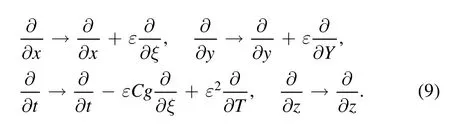
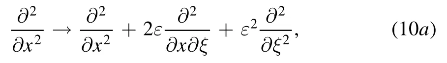
Noting the differential relations
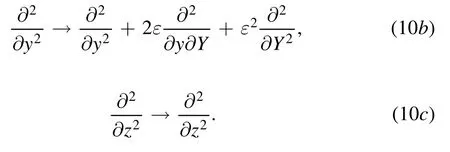
We introduce the following linear operator:
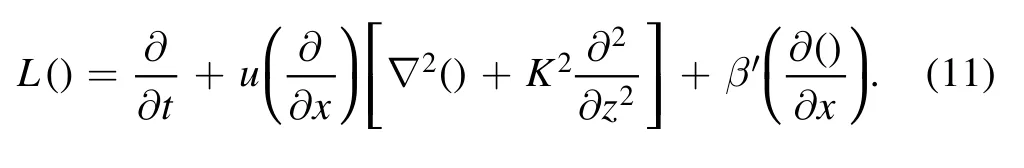
Substituting equations(8)–(10)into equation(7),we find that φ satisfies the equation
We assume that the solution of equation (12) is

where A is the Rossby wave amplitude, k and l are the dimensionless Rossby wavenumbers in the corresponding directions,

is the Rossby wave frequency, and Θ represents the complex conjugate of all the preceding terms.Substituting equation (13) into equation (12), we get
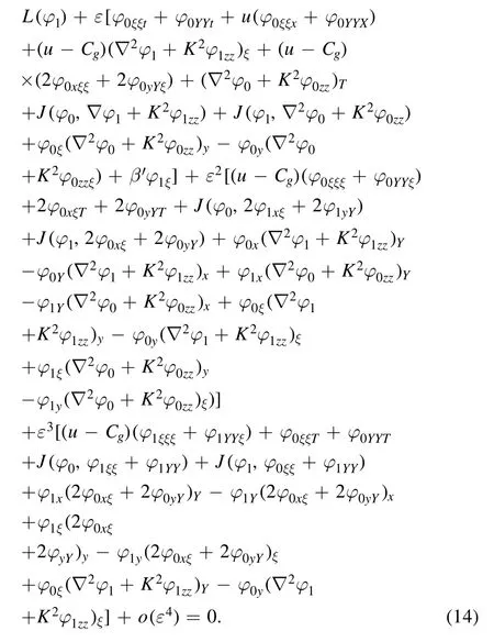
We suppose that equation (14) has a solution of the form

and that the solution φ can be expressed as
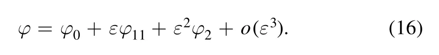
Here, φ11can be assumed to be given by [18]
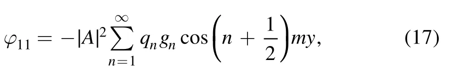
where qnand gnare coefficients.Substitution of equation(16)into equation (14) yields
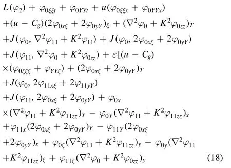
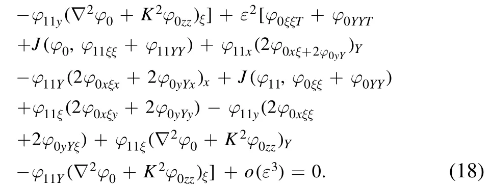
Substituting equations(13),(16),and(17)into equation(18),and eliminating exp [ i (kx+lz-ωt)], we obtain
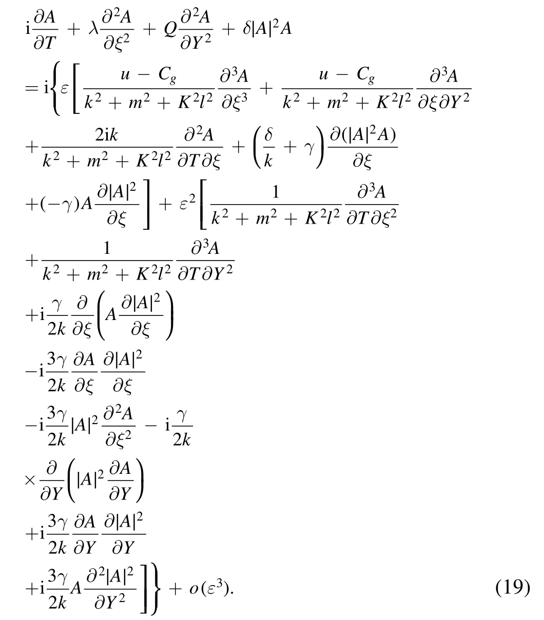
To simplify equation (19), we use i∂A/∂T to eliminate highorder terms ∂2A/∂T∂ξ, ∂3A/∂T∂ξ2, and ∂3A/∂T∂Y2.Thus,we arrive at a(2+1)-dimensional fourth-order NLS equation without complex high-order terms By ignoring the terms of order equal to or higher than O(ε3), we obtain the following high-order Schrödinger equation:
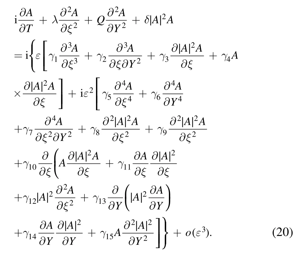
The coefficients in equations (19) and (20) are given in appendix A.Equation(20)is a new(2+1)-dimensional highorder NLS equation describing Rossby waves in stratified fluids.This fourth-order NLS equation represents an extension of the equations considered in previous studies to(2+1)dimensions.When ε=0 and Q=0, the equation reduces to the standard NLS equation.When ε=0 and Q ≠0,it reduces to the (2+1)-dimensional NLS equation.When O(ε2) and terms O(ε3) are ignored, the equation becomes a Sasa–Satsuma equation [34].When we do not consider terms O(ε3), the equation is the (2+1)-dimensional fourth-order NLS.In the case of the standard NLS equation, there have been many discussions of the modulational instability of uniform Rossby waves.Next, we will discuss the modulational instability of finite-amplitude Rossby waves using equation (19) with high-order terms O(ε) and O(ε2).
3.Modulational instability
Modulational instability occurs widely in nonlinear media and is responsible for a variety of physical phenomena.Owing to the influence of dispersion and nonlinear effects,initial stable continuous waves will become unstable during transmission,resulting in self-modulation of frequency and amplitude.
Here, we will focus on the modulational instability of uniform Rossby waves subjected to small disturbances in a two-dimensional space.Ignoring terms O(ε3)in equation(19), we consider its plane wave solution

where A0is a constant, representing the Rossby wave amplitude.Suppose that a small disturbance is superimposed on the Rossby waves, representing their modulation.We then have the following plane wave solution:

where ψ(ξ, Y, T) is the small disturbance.We substitute equation (22) into equation (19), and linearize the resulting equation.After some calculation, we obtain the following linearized equation for the small disturbance ψ(ξ, Y, T):
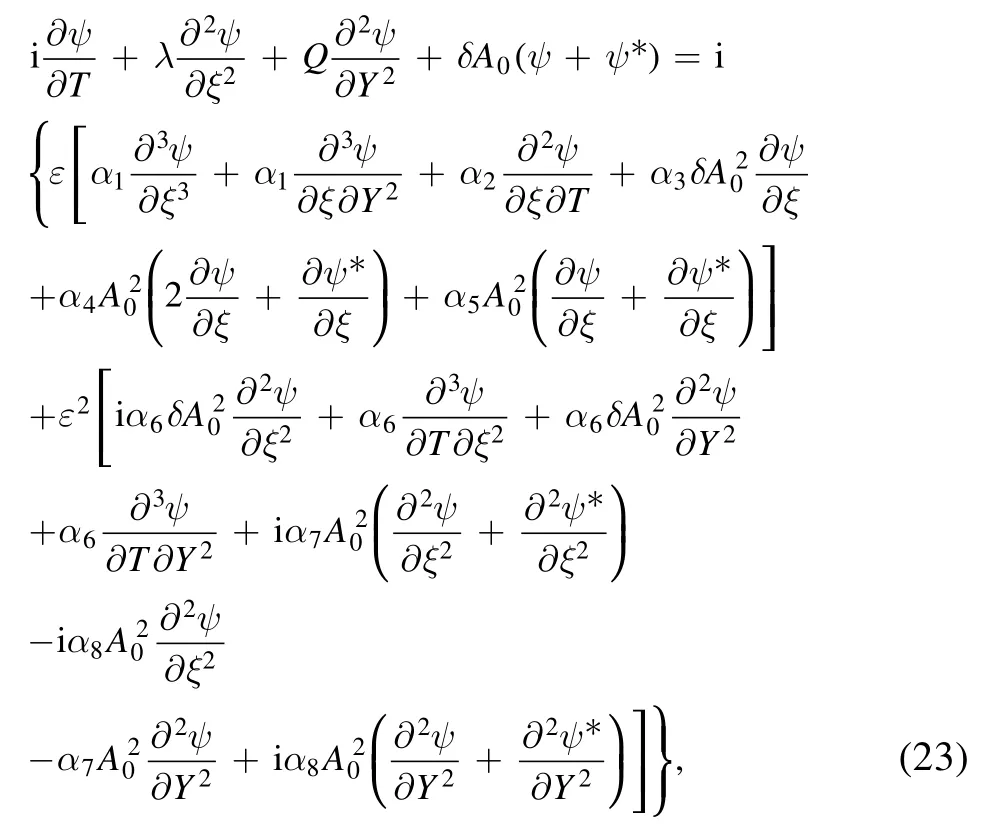
where the coefficients are given in appendix B.
Suppose that ψ has the following form:
Substituting equation (24) into equation (23), and separating the real and imaginary parts, we obtain the real part as
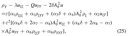
and the imaginary part as
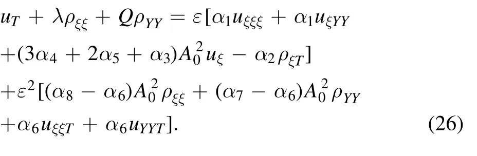
For periodic modulation, using the Euler’s formula, we can assume that the solutions are
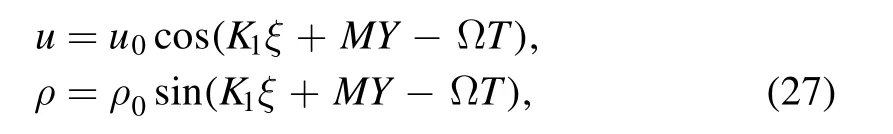
where u0and ρ0are constants, and K1and M represent the perturbation wavenumbers of the Rossby waves in the x and y directions, respectively.Substituting equation (27) into equations (25) and (26), we get a system of equations in matrix form for u0and ρ0:

For equation (28) to have a solution, the determinant of its coefficient matrix must be zero.To simplify equation(28),we define B0=εA0, εK1=pk, εM=qm, and Ω=W/ε2.Then,the following dispersion relation can be obtained:
where
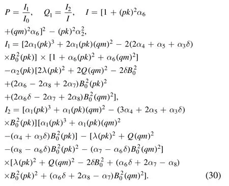
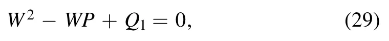
From equation (29), we have
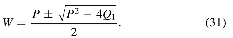
Thus, when P2−4Q1>0, the frequency Ω of the uniform Rossby waves is a real number,and so the waves are stable.When P2−4Q1<0, Ω is a complex number, and the uniform Rossby waves are unstable.In this case, there is modulation of the steady-state solution of the uniform Rossby waves, and we therefore call this phenomenon modulational instability.
The conditions for modulational instability of other types of NLS equation can also be obtained from equation(31).When αi(i=1,…,8)=0,we can obtain the conditions for modulational instability of the (2+1)-dimensional NLS equation.When αi(i=6, …, 8)=0, we can obtain the conditions for modulational instability of the third-order Hirota equation.Examination of equation (31)reveals that the dimension and order of the equation, the latitude at which the Rossby waves occur, and the uniform base flow all affect the modulational instability gain.When P2−4Q1<0, we define the modulational instability gain of uniform Rossby waves asG= 2 × 10⁻⁴× Im{W}.Next, we will discuss the factors that affect the modulational instability gain and region.
4.Factors affecting modulational instability
4.1.Dimension of equation
First of all, we consider the effect of dimension on the modulational instability gain.It is easy to see that since the disturbances superimposed on the x or y directions are different, the modulational instability gain of Rossby waves will be affected.We take the wavenumber p in the x direction as a variable.From the plots of modulational instability gain and regions of modulational instability and stability shown in figure 1, it can be seen that when only the dependence of the instability on p is considered,with the dependence on the wavenumber q in the y direction being ignored, the modulational instability gain is symmetrically distributed on both sides of p=0, i.e.the sign of p has no effect on the gain.This indicates that whether a superimposed small disturbance in the x direction is positive or negative has no effect on the modulational instability gain.With increasing |p|, the modulational instability gain first increases and then decreases, finally tending to zero.When p=0, G=0.When 0 <p <4.3 and −4.3 <p <0, the changes in gain with p are as shown in figure 1(a) and the distribution of regions of modulational instability are as shown in figure 1(b).When p >4.3 and p <−4.3,the modulational instability gain is 0.The modulated Rossby waves are then stable, and the regions of stability are also shown in figure 1(b).We now take account of the wavenumber q in the y direction.When we change the value of q, i.e.change the number of perturbed waves in the y direction,the modulational instability gain of Rossby waves at 60°N for Ly=5 is as shown in figure 2.It can be seen that when q=0, the instability occurs in the range |p|≤4.3 and the modulational instability gain becomes 0 at|p|=4.3,when q=0.2,the instability occurs in the range|p|≤4.29 and the gain becomes 0 at|p|=4.29, and when q=0.5, the instability occurs in the range |p|≤4.25 and the gain becomes 0 at |p|=4.25.For Ly=1, figure 3 shows that when q=0, the modulational instability occurs at |p|≤2.75, when q=0.2, the modulational instability occurs at |p|≤2.46, and when q=0.5, the modulational instability occurs at |p|≤1.4.This shows that with increasing wavenumber q in the y direction, the region of modulational instability of Rossby waves becomes narrower, and the modulational instability gain also changes.
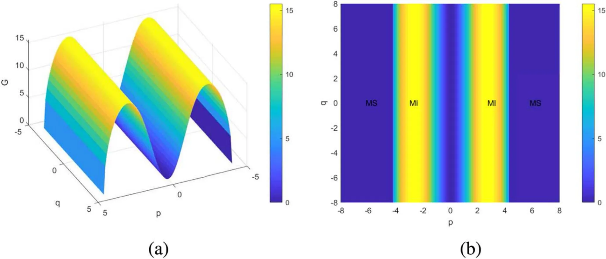
Figure 1.(a) Modulational instability gain G and (b) regions of modulational instability (MI) and modulational stability (MS) of Rossby waves at 60°N for k = 3 (6.371 cos 60° ), K=1, l=1, Ly=5, B0=0.5, and u=1.Here, only the dependence of the instability on the wavenumber p in the x direction is considered, with the dependence on the wavenumber q in the y direction being ignored.
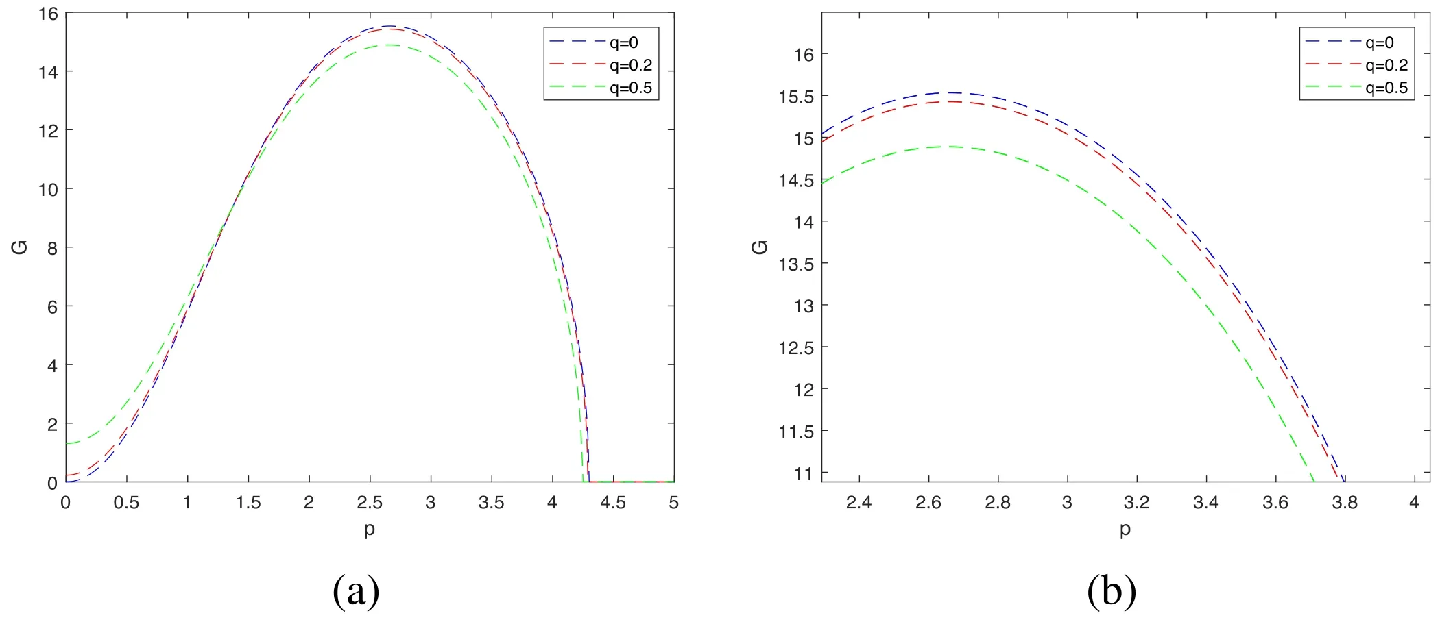
Figure 2.(a)Modulational instability gain G of Rossby waves at 60°N for q=0(blue curve),q=0.2(red curve),and q=0.5(green curve)for k = 3 /(6.371 cos 60 °), K=1, l=1, Ly=5, B0=0.5, and u=1.(b) Magnified view of part of the plot in (a).
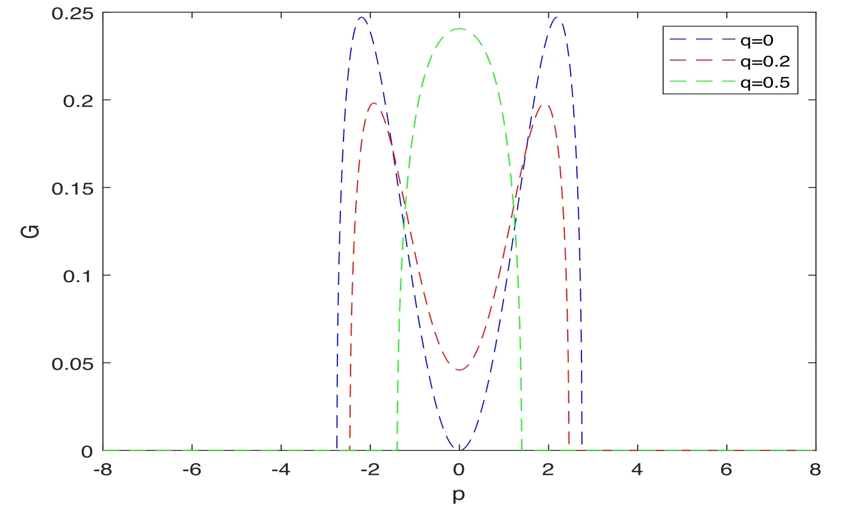
Figure 3.Modulational instability gain G of Rossby waves at 60°N for q=0(blue curve),q=0.2(red curve),and q=0.5(green curve)for k =3 /(6.371 cos 60° ), K=1, l=1, Ly=1, B0=0.5, and u=1.
We now take the wavenumber q in the y direction as a variable and consider the effect of the perturbation wave number p in the x direction on the variation of the modulational instability gain with the wavenumber q in the y direction, as shown in figure 4 for Rossby waves at 60°N.It can be seen that the modulational instability gain increases with increasing p, rapidly at first, then more slowly,and finally tending to a fixed value.The area above the curve corresponds to the modulationally stable region,and the area below the curve to the modulationally unstable region.
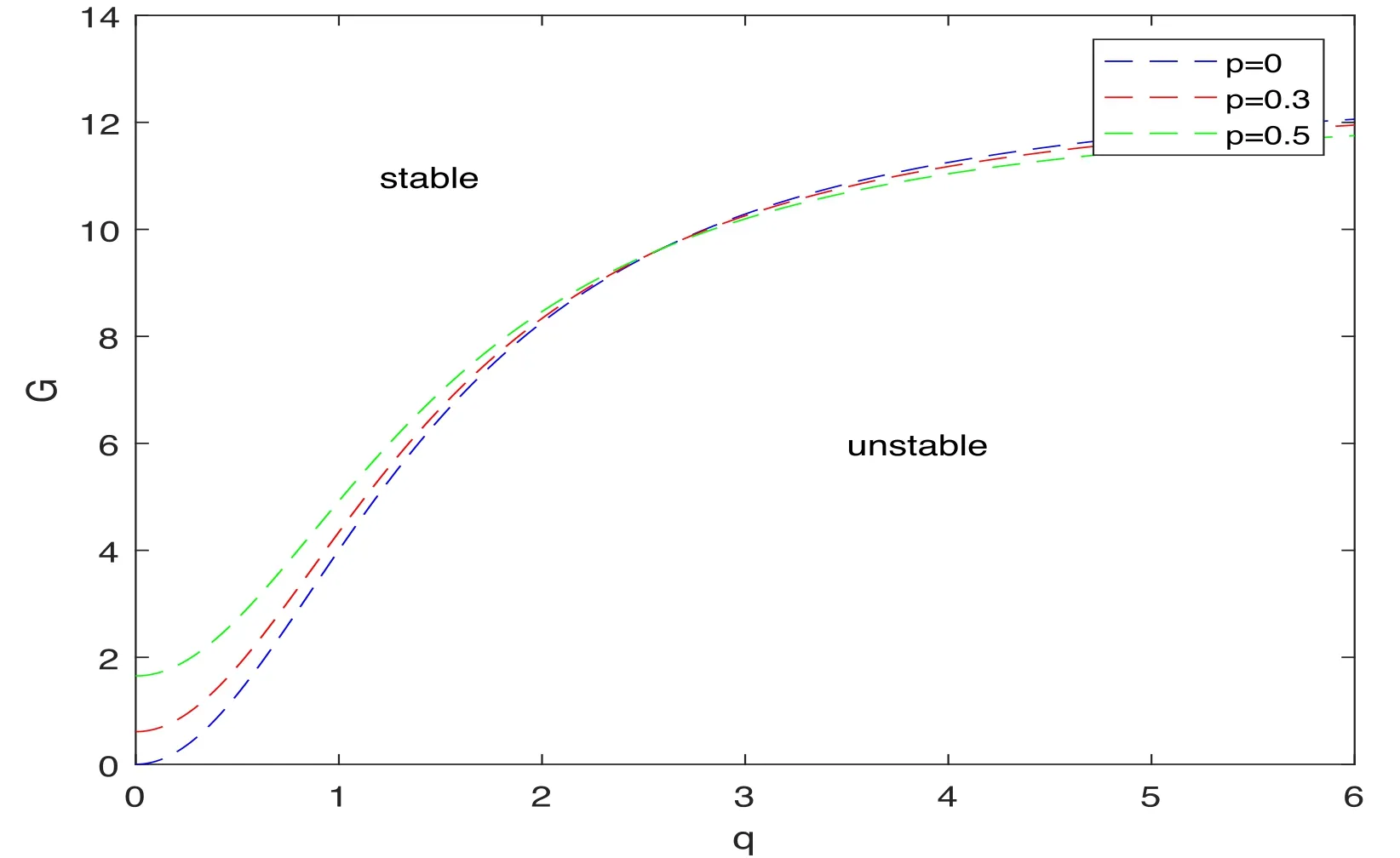
Figure 4.Modulational instability gain G of Rossby waves at 60°N for p=0(blue curve),p=0.3(red curve),and p=0.5(green curve)for k =3 /(6.371 cos 60° ), K=1, l=1, Ly=5, B0=0.5, and u=1.
Finally, we consider the combined effects of p and q on modulational instability of Rossby waves in two-dimensional space and show the changes in instability gain and regions of instability in figure 5.
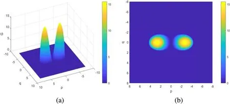
Figure 5.(a)Modulational instability gain G and(b)regions of modulational instability of Rossby waves at 60°N for k = 3 /(6.371 cos 60° ),K=1,l=1,Ly=5,B0=0.5,and u=1.Here,the dependences of the instability on both the wavenumbers p and q in the x and y directions,respectively, are considered.
In summary, we can conclude that the (1+1)-dimensional NLS equation can only describe changes in the modulational instability of Rossby waves in one direction,while the (2+1)-dimensional equation is able to describe these changes in both the x and y directions.When we change the number of disturbance waves in the direction of x or y,the modulational instability gain will be affected,and the regions of instability will also change.It is clear that these changes may affect the propagation and stability of Rossby waves.
4.2.Order of the NLS
We now compare the modulational instability gain according to the standard NLS equation and according to the high-order NLS equation to explore the effect of the high-order terms on the modulational instability of Rossby waves.The standard(2+1)-dimensional NLS equation has the following form:
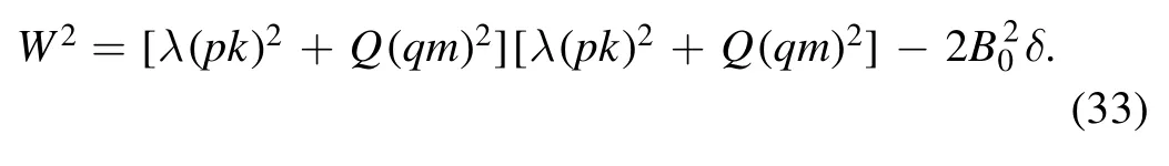
From equation(31),we can easily obtain the expression for the modulational instability of this equation as
Without loss of generality, we take p as the variable and fix q=0.01.Figure 6 shows the variation of the modulational instability gain of Rossby waves with the wavenumber p.Taking figure 6(b) as an example, we can see that for the standard NLS,the Rossby waves are modulationally unstable in the range 0 <p <4.54 and stable in the range p >4.54.For the (2+1)-dimensional high-order NLS, the Rossby waves are modulationally unstable when 0 <p <4.3 and stable when p >4.3.Thus,we can see that when p is greater than a certain value, the modulational instability gain of Rossby waves with high-order terms αiis smaller than that in the absence of high-order terms.The region of modulational instability is narrower when high-order terms αiare present than when they are absent.This shows that high-order terms will affect the modulational instability of Rossby waves, and taking these terms into account enables a more accurate determination of the regions where modulational instability occurs.Therefore, in general, the inclusion of high-order terms gives a better representation of the modulational instability of Rossby waves.
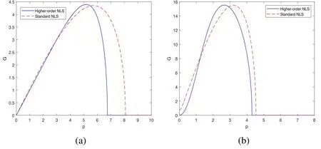
Figure 6.Modulational instability gain G according to the(2+1)dimensional higher-order NLS(blue full curves)and the standard NLS(red dashed curves) for K=1, l=1, B0=0.5, k = 3/ (6.371 cos 60° ), and (a) Ly=0.1, (b) Ly=5.
4.3.Latitude at which Rossby waves occur
We now discuss the changes in the modulational instability of Rossby waves when the latitude at which the waves occur changes.From the point of view of the equation describing the Rossby waves, because the zonal wavenumber k is directly related to the latitude, k is larger at higher latitudes and smaller at lower latitudes.Therefore, the modulational instability of Rossby waves will be different at different latitudes.To reveal the changes in instability gain caused by changes in latitude, we take q=0.01 and compare the modulational instability of Rossby waves at latitudes of 50°N and 60°N, respectively, as shown in figure 7.Taking figure 7(b)as an example, we can see that for latitude 50°N, the modulationally stable region of Rossby waves corresponds to p >4.36 and the modulationally unstable region to 0 <p <4.36.For latitude 60°N, the modulationally stable region corresponds to p >5.16 and the modulationally unstable region to 0 <p <5.16.Similar differences can be seen in figure 7(a).Thus, under the same conditions, it is found that when only a change in latitude is considered, the region of modulational instability of Rossby waves at latitude 50°N is narrower than at latitude 60°N.However, as can be seen from figure 7, the trend of variation of the modulational instability gain at the two latitudes is the same.
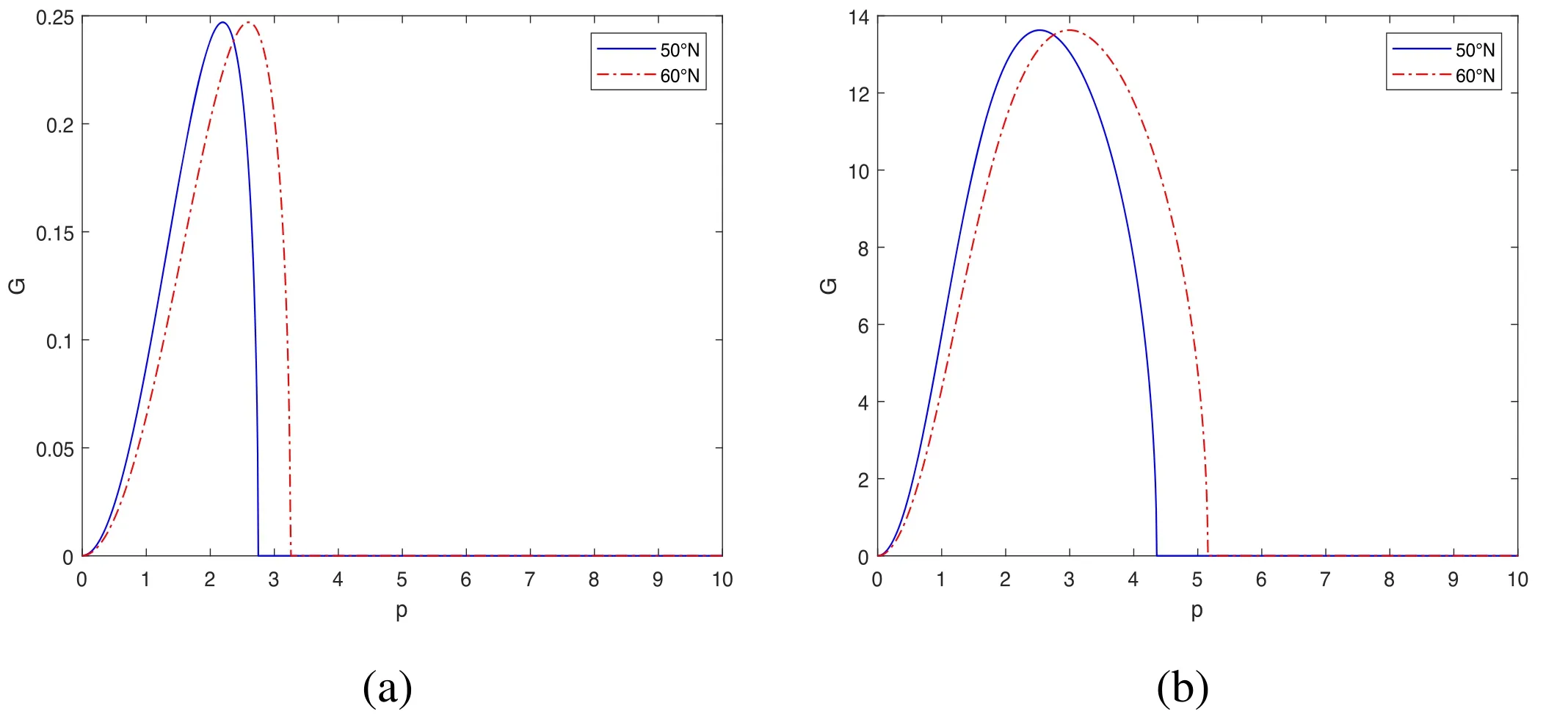
Figure 7.Comparison of modulational instability gain of Rossby waves at latitudes of 50°N and 60°N for K=1, l=1, B0=0.5,k1 =3/ (6.371 cos 50°), k2 = 3 /(6.371 cos 60°), and (a) Ly=1, (b) Ly=5.
We can conclude that for Rossby waves under the same background conditions,modulational instability is more likely to occur at high latitudes.This is because nonlinear effects on the behavior of large-scale waves, especially planetary-scale waves, are more prominent in high-latitude regions.Therefore,the(2+1)-dimensional high-order NLS equation will be more suitable for describing nonlinear Rossby waves at high latitudes.
Various studies have shown that in addition to the dimension and order of the NLS equation and the latitude at which Rossby waves occur, their modulational instability is affected by other factors that have not been considered here,such as amplitude and topography.Moreover, this study has not discussed the effect of external forces and frictional dissipation on modulational instability, which are topics that deserve further study.
5.Conclusion
By using an iterative perturbation method and a multiscale analysis,we have derived a new(2+1)-dimensional high-order NLS equation containing terms O(ε) and O(ε2) for Rossby waves in stratified fluids.Using this equation, we have studied the modulational instability of Rossby waves and have obtained conditions for their modulational instability.The results show that the Rossby waves are stable when P2−4Q1>0 and unstable when P2−4Q1<0.On this basis, we have further discussed the factors affecting the modulational instability of Rossby waves, mainly considering the effects of the dimension and order of the NLS equation and the effect of the latitude at which the waves occur on the instability gain and region of instability.Our theoretical analysis and numerical simulations have led us to the following conclusions:
1.The(2+1)-dimensional NLS equation can describe the changes of modulational instability of Rossby waves in two-dimensional space.Increasing the number of disturbance waves in different directions will affect the modulational instability gain, and the regions of instability will also change.The (2+1)-dimensional NLS equation provides a more accurate description of the modulational instability of Rossby waves than the standard (1+1)-dimensional equation.
2.When the disturbance wavenumber is large, the modulational instability gain of Rossby waves with high-order terms αiis smaller than in the absence of such terms.When high-order terms are taken into account, the region of modulational instability is narrower.This shows that high-order terms can affect the modulational instability of Rossby waves, and the inclusion of these terms gives a more accurate description of the growth of modulational instability.
3.The region of modulational instability of Rossby waves at latitude 50°N is narrower than at latitude 60°N.This shows that Rossby waves at high latitudes are more prone to modulational instability.
In summary,we have found that the(2+1)-dimensional high-order NLS equation is more suitable than the standard equation for describing Rossby waves in stratified fluids, and it can more accurately reflect changes in modulational instability in two-dimensional space.However,there is a need for further studies to take account of the effects of amplitude,external forces, topography, and other factors on Rossby waves and their modulational instability.
Acknowledgments
This work was supported by the National Natural Science Foundation of China (No.11975143).
Appendix A.Coefficients in equations (19) and (20)
Appendix B.Coefficients in equation (23)
猜你喜欢
儿童故事画报·自然探秘(2022年3期)2022-04-27
小学生学习指导(高年级)(2021年10期)2021-11-24
疯狂英语·新悦读(2021年5期)2021-06-08
阅读(快乐英语高年级)(2021年2期)2021-04-26
阅读(快乐英语中年级)(2020年11期)2020-12-28
艺术启蒙(2020年12期)2020-12-24
作文评点报·低幼版(2020年32期)2020-07-23
青年生活(2019年3期)2019-09-10
儿童故事画报·自然探秘(2019年10期)2019-01-14
电影文学(2018年14期)2018-12-09
 Communications in Theoretical Physics2022年7期
- Communications in Theoretical Physics的其它文章
- Stable striped state in a rotating twodimensional spin–orbit coupled spin-1/2 Bose–Einstein condensate
- The pseudoscalar meson and baryon octet interaction with strangeness S = -2 in the unitary coupled-channel approximation
- A new effective potential for deuteron
- Density fluctuations of two-dimensional active-passive mixtures
- Anisotropic and valley-resolved beamsplitter based on a tilted Dirac system
- Topological and dynamical phase transitions in the Su–Schrieffer–Heeger model with quasiperiodic and long-range hoppings