LIMIT CYCLES OF THE GENERALIZED POLYNOMIAL LI´ENARD DIFFERENTIAL SYSTEMS∗

Amel Boulfoul

（Dept.of Math.，20 August 1955 University，BP26，El Hadaiek 21000，Skikda.Algeria）

Amar Makhlouf

（Dept.of Math.，LMA Laboratory，Badji Mokhtar University，BP12，El Hadjar 23000，Annaba.Algeria）



LIMIT CYCLES OF THE GENERALIZED POLYNOMIAL LI´ENARD DIFFERENTIAL SYSTEMS∗

Amel Boulfoul†

（Dept.of Math.，20 August 1955 University，BP26，El Hadaiek 21000，Skikda.Algeria）

Amar Makhlouf

（Dept.of Math.，LMA Laboratory，Badji Mokhtar University，BP12，El Hadjar 23000，Annaba.Algeria）

Abstract

Using the averaging theory of first and second order we study the maximum number of limit cycles of generalized Li´enard differential systems

which bifurcate from the periodic orbits of the linear centerwhere ϵ is a small parameter.The polynomialsandhave degree l；andhave degree n；andhave degree m.p∈N and［·］denotes the integer part function.

limit cycle；periodic orbit；Li´enard differential system；averaging theory

2000 Mathematics Subject Classification 34C29；34C25；47H11

1　Introduction and Statement of the Main Results

One of the main problems in the theory of differential systems is the study of the existence，number and stability of limit cycles.A limit cycle of a differential system is an isolated periodic orbit in the set of all periodic orbits of the differential system.These last years hundreds of papers have studied the limit cycles of planar polynomial differential systems.The main reason of these studies is the unsolved 16thHilbert problem，see［7，8，10］.In this paper，we will try to give a partial answer to this problem for the class of generalized Li´enard polynomial differential system given by

where h（x），f（x）and g（x）are polynomials in the variable x of degree l，n and m respectively and p∈N.This system was studied when h（x）=0 in［1］.［12］and［13］considered the similar case of differential system（1）for p=0.

Note that when h（x）=g（x）=0 and p=0 system（1）coincides with the classical polynomial Li´enard differential system

where f（x）is a polynomial in the variable x of degree n.A generalization of classical Li´enard differential system（2）is the following system

where f（x）and g（x）are polynomials in the variable x of degree n and m respectively. We denote by H（m，n）the maximum number of limit cycles of system（3）.This number is usually called the Hilbert number for system（3）.

·In 1928，Li´enard［14］proved that if m=1 and F（x）=∫x0f（s）ds is a continuous odd function，which has a unique root at x=a and is monotone increasing for x≥a，then system（3）has a unique limit cycle.

·In 1973，Rychkov［19］proved that if m=1 and f（x）is an odd polynomial of degree five，then system（3）has at most two limit cycles.

·In 1977，Lins de Melo and Pugh［15］proved that H（1，1）=0 and H（1，2）=1.

·In 1988，Coppel［5］proved that H（2，1）=1.

·In 1997，Dumortier and Li［6］proved that H（3，1）=1.

·In 2012，Li and Llibre［11］proved that H（1，3）=1.

A well known method for obtaining results on the limit cycles of polynomial differential systems perturbs the linear center˙x=y，˙y=-x inside the class of polynomial differential systems，or inside the class of classical polynomial Li´enard differential systems.The limit cycles obtained in this way are sometimes called medium amplitude limit cycles.

In 2010，Llibre，Mereu and Teixeira［16］studied how many limit cyclescan bifurcate from the periodic orbits of the linear center to system（3）using the averaging theory.In fact they compute lower estimations ofMore precisely they compute the maximum number of limit cycleswhich bifurcate from the periodic orbits of the linear centerusing the averaging theory of order k，for k=1，2，3.For the limit cycles obtained by bifurcation of the orbits of the center of the Li´enard differential systems，see［4，18，22］.

In this work，we provide estimations offor all l，m，n≥1 computingfor k=1，2.Of course

Let k be a positive integer.We define ev（k）as the largest even integer≤k，and od（k）as the largest odd integer≤k.

First we consider system（1）withand g（x）=We obtain the following system

Theorem 1 For|ϵ|＞0 sufficiently small，the maximum number of limit cycles of the generalized polynomial Li´enard differential systems（4）bifurcating from the periodic orbits of linear center˙x=y，˙y=-x，using the averaging theory of first order is：

（a）For p=0，

（b）For p≥1，we have three cases：

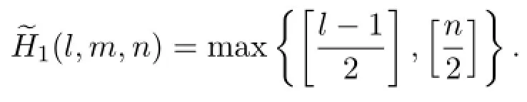
（i）If 1≤od（l）＜2p+1，

（ii）If 2p+1≤od（l）＜ev（n）+2p+1，

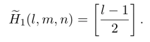
（iii）If od（l）≥ev（n）+2p+1，The proof of Theorem 1 is given in Section 3. Now we consider system（1）with

We obtain the following system

Theorem 2 For|ϵ|＞0 sufficiently small，the maximum number of limit cycles of the generalized polynomial Li´enard differential systems（5）bifurcating from the periodic orbits of linear center˙x=y，˙y=-x，using the averaging theory of second order is：

（a）For p=0，

（b）For p≥1，we have three cases to be considered：

（i）If 0≤σ1＜2p，

（ii）If 2p≤σ1≤σ2+2p，

（iii）If σ1＞σ2+2p，

where

The proof of Theorem 2 is given in Section 4.

In Section 2，we introduce the averaging theory of first and second orders.

2　Averaging Theory of First and Second Orders

Theorem 3 We consider the following differential system

where F1，F2：R×D→R，R：R×D×（-ϵf，ϵf）→R are continuous，T-periodic in the first variable，and D is an open subset of R.Assume that the following hypotheses（i），（ii）hold.

（i）F1（t，·）∈C2（D），F2（t，·）∈C1（D）for all t∈R，F1，F2，R are locally Lipschitz with respect to x，and R is twice differentiable with respect to ϵ.

We define Fk0：D→R for k=1，2 as

where

（ii）For V⊂D an open and bounded set and for each ϵ∈（-ϵf，ϵf）｛0｝，there exists an a∈V such that F10（a）+ϵF20（a）=0 and dB（F10+ϵF20，V，a）0.The expression dB（F10+ϵF20，V，a）/0 means that the Brouwer degree（see［2］）of the function F10+ϵF20：V→R at the fixed point a is not zero.A sufficient condition for the inequality to be true is that the Jacobian of the function F10+ϵF20at a is not zero.

Then，for|ϵ|＞0 sufficiently small there exists a T-periodic solution φ（·，ϵ）of the equation（6）such that φ（0，ϵ）→a when ϵ→0.

If F10is not identically zero，then the zeros of F10+ϵF20are mainly the zeros of F10for ϵ sufficiently small.In this case the previous result provides the averaging theory of first order.

If F10is identically zero and F20is not identically zero，then the zeros of F10+ ϵF20are mainly the zeros of F20for ϵ sufficiently small.In this case the previous result provides the averaging theory of second order.

For a general introduction to averaging theory see［3，20，21］.

3　Proof of Theorem 1

In order to apply the first order averaging method we write system（4）in polar

coordinates（r，θ）where x=rcosθ，y=rsinθ，r＞0.If we takeand，system（4）can be written in the following way

If we take θ as a new independent variable，this system becomes

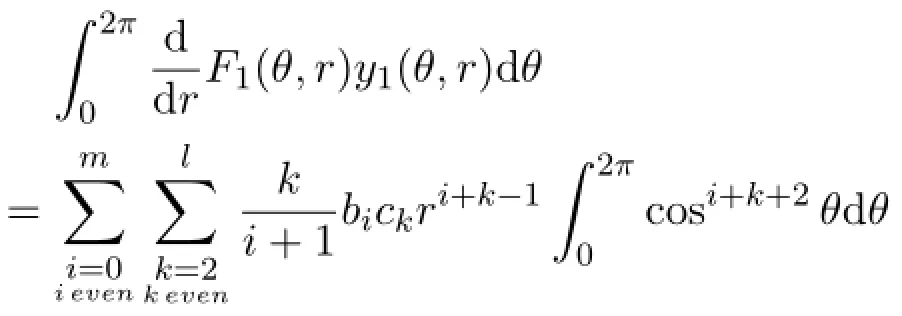
By using the notation introduced in Section 2 we have that

In order to calculate the exact expression of F10，we use the following formulas

where（2p+1）！！=1·3·5···（2p+1）.

Hence

（a）For p=0，we have that

Note that in order to find positive roots of F10，we must find the zeros of a polynomial in the variable r2of degree equal to

（b）For p≥1，we distinguish three cases：

（i）If 1≤od（l）＜2p+1，

The maximum number of positive roots of a polynomial in r2in this case is

（ii）If 2p+1≤od（l）＜ev（n）+2p+1，

In this case，The polynomial F10has at most

real positive roots.

（iii）If od（l）＞ev（n）+2p+1，

4　Proof of Theorem 2

For proving Theorem 2 we shall use the second order averaging theory.We consider the differential system（5）

where

Then system（5）in polar coordinates（r，θ），r＞0 becomes

Now taking θ as a new independent variable，system（5）becomes

Now we determine the corresponding function

For this we put F10≡0 which is equivalent to

First，we have that

and

where

and

For more details see［9］.

So

Moreover

Then F20is the polynomial

where

and

（a）For p=0，equation（8）becomes

This polynomial has at most

real positive roots.

（b）For p≥1，we denote by

σ1=max｛ev（l）+ev（m）-2，od（l）-1｝and σ2=max｛od（n）+ev（m）-1，ev（n）｝. Note that

so，we have three cases：

（i）If 0≤σ1＜2p，in this case equation（8）can be written as

This polynomial has at most

real potive roots.

（ii）If 2p≤σ1≤σ2+2p，

The maximum number of positive real roots that can has F20is at most

（iii）If σ1≥σ2+2p，the polynomial F20is

which has at most

positive roots.Hence Theorem 2 follows.

References

［1］A.Boulfoul&A.Makhlouf，Limit cycles of the generalized polynomial Li´enard differential equations，Ann.of Diff.Eqs.，28（2012），127-131.

［2］F.Browder，Fixed point theory and nonlinear problems，Bull.Amer.Math.Soc.，9（1983），1-39.

［3］A.Buic˘a&J.Llibre，Averaging methods for finding periodic orbits via Brouwer degree，Bull.Sci.Math.，128（2004），7-22.

［4］A.Gasull&J.Torregrosa，Small-amplitude limit cycles in Li´enard systems via multiplicity，J.Diff.Eqs.，159（1998），1015-1039.

［5］W.A.Coppel，Some quadratic systems with at most one limit cycles，In Dynamics reported，New York：Wiley，2（1998），61-68.

［6］F.Dumortier&C.Li，Quadratic Li´enard equations with quadratic damping，J.Diff. Eqs.，139（1997），41-59.

［7］D.Hilbert，Mathematische probleme，lecture in：secondInternat.Cong.Math，Paris，1900，Nachr.Ges.Wiss.G¨ottingen.Math.Phys.Ki 5（1900），253-297；English Transl：Bull.Amer.Math.Soc.，8（1902），437-479.

［8］Y.Ilyashenko，Centennial history of Hilbert's 16th problem，Bull.Amer.Math.Soc.，39（2002），301-354.

［9］I.S.Gradshteyn&I.M.Ryzhik，Table of Integrals，Series and Products，Academic Press，1979.

［10］Jibin Li，Hilbert's 16th problem and bifurcations of planar polynomial vector fields，Internat.J.Bifur.Chaos.Appl.Sci.Engrg.，13（2003），47-106.

［11］C.Li&J.Llibre，Uniqueness of limit cycle for Li´enard equations of degree four，J. Diff.Eqs.，252（2012），3142-3162.

［12］J.Llibre&C.Valls，On the number of limit cycles of a class of polynomial differential systems，Proc.R.Soc.A，468（2012），2347-2360.

［13］J.Llibre&C.Valls，On the number of limit cycles for a generalization of Li´enard polynomial differential systems，Int.J.Bifurcation Chaos，23（2013），16pp.

［14］A.Li´enard，´Etude des oscillations entrenues，Rev.G´en.´Electricit´e，23（1928），946-954.

［15］A.Lins，W.de Melo&C.C.Pugh，On Li´enard's equation，Lecture Notes in Mathematics，597（1977），335-357，Berlin，Germany：Springer.

［16］J.Llibre，A.C.Mereu&M.A.Teixeira，Limit cycles of the generalized polynomial Li´enard differential equations，Math.Proc.Camb.Phil.Soc.，148（2010），363-383.

［17］N.G.Lloyd，Limit cycles of polynomial systems-some recent developments，London Math.Soc.Lecture Note，Cambridge University Press，127（1988），192-234.

［18］N.G.Lloyd&S.Lynch，Small-amplitude limit cycles of certain Li´enard systems，Proc. Royal Soc.London Ser.A，418（1988），199-208.

［19］G.S.Rychkov，The maximum number of limit cycle of the system ˙x=y-a1x3-a2x5，˙y=-x is two，Diff.Uravneniya，11（1975），380-391.

［20］J.A.Sanders&F.Verhust，Averaging methods in nonlinear dynamical systems，Applied Mathematical Sci.，Vol.59，Springer-Verlag，New York，1985.

［21］F.Verhulst，Nonlinear differential equations and dynamical systems，Berlin：Springer-Verlag，Second Edition，1991.

［22］P.Yu&M.Han，Limit cycles in generalized Li´enard systems，Chaos，Solitons and Fractals，30（2006），1048-1068.

（edited by Mengxin He）

∗Manuscript received March 24，2016；Revised May 12，2016†Corresponding author.E-mail：a.boulfoul@univ-skikda.dz