
L6BOUND FOR BOLTZMANN DIFFUSIVE LIMIT∗
2016-10-14 02:40YanGuo
Annals of Applied Mathematics 2016年3期
Yan Guo
(Division of Applied Math.,Brown University)
L6BOUND FOR BOLTZMANN DIFFUSIVE LIMIT∗
Yan Guo†
(Division of Applied Math.,Brown University)
Abstract
We consider diffusive limit of the Boltzmann equation in a periodic box. We establish L6estimate for the hydrodynamic part Pf of particle distribution function,which leads to uniform bounds global in time.
L6estimate;Boltzmann equation;diffusive limit
2000 Mathematics Subject Classification 76P05
1 Introduction
We study the diffusive limit of the Boltzmann equation

with the particle distribution functionin a periodic box of T3×R3,whereis a normalized Maxwellian.For simplicity, we assume the collision operator Q is given by the classical hard-sphere interaction. In terms of perturbation f,we have

We denote the hydrodynamic part of f(t,x,v)


where[u(t,x),θ(t,x)]satisfies the celebrated incompressible Navier-Fourier system

with Boussineq approximation ρ+θ=0,see[3].
As in many singular perturbation problems[3],the key is to obtain uniform estimates for solutions to the Boltzmann equation(1).In[3],a nonlinear energy method leads to uniform bounds in high Sobolev norms.A natural question left open was whether one can obtain uniform bounds with lower regularity.This is particularly important in the study of boundary value problem [1,2,4],in which high Sobolev regularity is impossible in general.
As in[1],we establish uniform bounds without any Sobolev regularity in this paper.The main idea is to start with basic energy estimate,which leads to control of the microscopic(kinetic)part

where the collision frequency ν(v)~〈v〉,for the hard-sphere case.By the positivity estimate in[4],the macroscopic partcan be controlled.Unfortunately, such abound is not strong enough to control the nonlinearity Γ(f,f)uniformly in ε.The main novelty is to obtain uniform estimates in ε for Pf with an improved L6estimate for the macroscopic part Pf.This new estimate leads to an improved L∞bound,which completes the control of Γ(f,f).
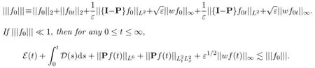
We now define energy E(t)and dissipation rate D(t)as

Our main result consists of the following a-priori uniform estimate.
Theorem 1Assume hard-sphere collision kernel.Assume f is a solution to the Boltzmann equation (1).Letsome l≫1,
2 Energy Estimate
The starting point is the following natural energy estimate.
Lemma 1 For solution f to(1),we have

The proof of this lemma follows from taking L2-inner product(·,·)x,vof f with
(1),and of∂tf with∂t×(1),as well as using the positivity of[4]

and the collision invariance

To control the nonlinear terms in(2),it is important to control higherintegrability of Pf.
Lemma 2 Assume that g solves

Proof The proof is an improvement ofestimates in[2].The key is to choose appropriate test function ϕ similar to that in[2]for the weak formulation of(1),by keepingbounded.
Recall


and βcis to be determined.We remark that by Sobolev's imbedding and W2,pelliptic theory in 3D,

We have from the periodicity and the Green's identity(weak formulation of(1))that


We choose βc

so that the contribution of a vanishes inTherefore,

thanks toc=0.On the other hand,

We therefore conclude the estimate for c(t,x)as

Estimate of b.We define ϕbas


We first choose test function ofto(3)and obtain

where we have set βbsuch that for any i

so that direct computation yields for ik

As in the estimate for c,it thus follows that

On the other hand,we then chooseto obtain in(3)


Therefore,we conclude fromb=0,

Estimate of a.We choose


where βais determined by

to eliminate contribution from c,and our lemma follows.The proof is complete.
Lemma 3 Assume that g solves


Proof The key of the proof is to use the similar choices of test functions(with extra dependence on time)and estimate the new contributionin the time dependent weak formulation

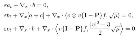
We note that,with such choicesand
From the conservation of mass,momentum and energy,we have

Step 2Estimate of c.
To estimate c,we define where ϕcis periodic and satisfies

We then plug the test function

into(12).We first note:

The second line has non-zero contribution only for j=i which leads to zero by the choosing of βsuch thatin(4).We have

Next,we treat the main term

Thanks to the definition of βc,we deduce

We conclude

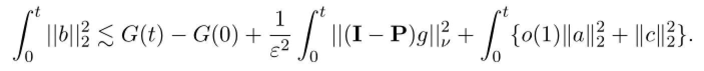
Step 3Estimate of b.
To estimate b,we define ϕbas


Similar to(5)and(7),we obtain


We repeat(8)and(9)to get for

We therefore conclude
Step 4Estimate for a.
To estimate a,we define

Choose test function ψ

in(12).We estimate

Together with(10),we conclude

Combining all the estimates and choosing o(1)small,we complete the proof.
4 L∞Estimate
We also need L∞estimate to control the nonlinearity in the energy estimate.
Lemma 4 Assume g solves

then for some weight w(v)=〈v〉lsome large l>1,

Proof Recall L=ν(v)-K.We rewrite for wg=q,


The first term is bounded byand the third term is bounded bysince ν(v)~〈v〉.We repeat such an expression foragain to evaluate the second term as

We now concentrate on the main contribution of the second term.We bounded it by the following pieces:


The first main contribution is bounded by

where

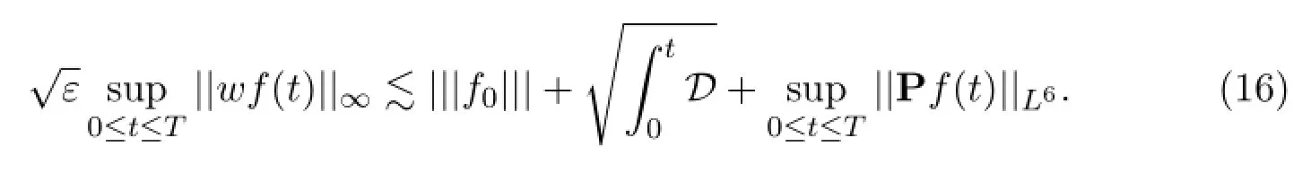
We now estimate the L6norm as

so that

and the L6norm is bounded by

5 Nonlinear Estimates
Lemma 5 Let f be a solution to the Boltzmann equation(1),then

Proof We apply Lemma 4 to(1)with h=Γ(f,f),


Therefore,

We now estimate Pf by applying Lemma 2 to

so that


We therefore have

Combining with(16),we deduce our lemma.
Lemma 6 Let f be a solution to the Boltzmann equation(1),then there existandwith

such that the following estimates are valid:


and

We note that


By multiplying a cut off function χ(t)beyond t≤0 if necessary,we deduce from the ε-averaging lemma[5]that,for some

Furthermore,

We note that from Lemma 3 to both(1)and∂t×(1)


Finally,we split


Hence,we may define

Clearly(18)follows from(20).Same splitting(21)for[at,bt,ct]leads to(19).The proof is complete.
Lemma 7 Let f be a solution to the Boltzmann equation(1),if

then

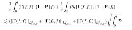
Proof We first split Γ(f,f),Γ(ft,f)and Γ(f,ft)into


On the other hand,from(18)and(19),

so that

We conclude our lemma from(15)

The proof is complete.
Proof of the Theorem 1 In the energy estimate(2),if

then we deduce


and(13)together with a standard continuity argument lead to

Acknowledgements This work grows out of[1].Yan Guo's research is supported in part by NSF grant No.1209437 and NSF of China grant No.10828103,as well as a Simon Fellowship.
References
[1]R.Espositio,Y.Guo,C.Kim,R.Marra,Stationary solutions to the Boltzmann equation in the hydrodynamic limit,arXiv:1502.05324
[2]R.Esposito,Y.Guo,C.Kim,R.Marra,Non-isothermal boundary in the Boltzmann theory and Fourier law,Comm.Math.Phys.,323(2013),177-239.
[3]Y.Guo,Boltzmann diffusive limit beyond the Navier-Stokes approximation,Comm. Pure and Appl.Math.,59(2006),626-687.
[4]Y.Guo,Decay and continuity of the Boltzmann equation in bounded domains,Arch. Ration.Mech.Anal.,197(2010),713-809.
[5]L.Saint-Raymond,Hydrodynamic limits of the Boltzmann equation,Lecture Notes in Mathematics,no.1971.Springer-Verlag,Berlin,2009.
(edited by Liangwei Huang)
∗Manuscript received July 6,2016
†Corresponding author.E-mail:yan guo@brown.edu
 Annals of Applied Mathematics2016年3期
- Annals of Applied Mathematics的其它文章
- LIMIT CYCLES OF THE GENERALIZED POLYNOMIAL LI´ENARD DIFFERENTIAL SYSTEMS∗
- SCALE-TYPE STABILITY FOR NEURAL NETWORKS WITH UNBOUNDED TIME-VARYING DELAYS∗†
- EFFECTS OF A TOXICANT ON A SINGLE-SPECIES POPULATION WITH PARTIAL POLLUTION TOLERANCE IN A POLLUTED ENVIRONMENT∗†
- OPTIMAL DECAY RATE OF THE COMPRESSIBLE QUANTUM NAVIER-STOKES EQUATIONS∗†
- BIFURCATIONS AND NEW EXACT TRAVELLING WAVE SOLUTIONS OF THE COUPLED NONLINEAR SCHR¨ODINGER-KdV EQUATIONS∗
- ALTERING CONNECTIVITY WITH LARGE DEFORMATION MESH FOR LAGRANGIAN METHOD AND ITS APPLICATION IN MULTIPLE MATERIAL SIMULATION∗†