
Investigation of the hydrodynamic performance of crablike robot swimming leg *
2018-09-28 05:34LiquanWang王立权HailongWang王海龙GangWang王刚XiChen陈曦AskerKhanLixingJin靳励行
水动力学研究与进展 B辑 2018年4期
Li-quan Wang (王立权), Hai-long Wang (王海龙), Gang Wang (王刚), Xi Chen (陈曦), Asker Khan ,Li-xing Jin (靳励行)
1. College of Mechanical and Electrical Engineering, Harbin Engineering University, Harbin 150001, China
2. State Key Laboratory of Autonomous Underwater Vehicle, Harbin Engineering University, Harbin 150001,China
3. College of Mechanical and Electrical Engineering, Heilongjiang Institute of Technology, Harbin 150001,China
Abstract: The existing amphibious robots cannot usually enjoy a superior adaptability in the underwater environment by replacing the actuators. Based on the bionic prototype of the Portunus trituberculatus, a new leg-paddle coupling crablike robot with a composite propulsion of walking legs and swimming legs is developed, with both the abilities of walking and swimming under water.By simulation and experiment, the effects of the phase difference, the flapping amplitude and the angular bias of the coupling movement, as well as the Strouhal number on the hydrodynamic performance of the swimming legs are studied, and the time dependent tail vortex shedding structure in a cycle is obtained. Both experimental and numerical results indicate that the thrust force with a high propulsion efficiency can be generated by a flapping swimming leg. This work can further be used for analysis of the stability and the maneuverability of the swimming leg actuated underwater vehicles.
Key words: Leg-paddle coupling crablike robot, swimming leg, hydrofoil propulsion, hydrodynamic performance
Introduction
Various kinds of unmanned underwater vehicles were developed for the marine industry. The traditional underwater vehicles equipped with propulsive propellers show low propulsive efficiency and poor maneuverability[1]. The bionic propulsion enjoys many advantages, including low noise and lesser resistance, good concealing ability, strong adaptability,low cost and mass production, therefore, has broad application prospects in the field of underwater vehicles[2]. According to their propulsion methods of imitating underwater creatures, the propulsions of the existing bionic underwater vehicles can be classified as: the bionic fish oscillating propulsion, the bionic squid jet propulsion, the bionic multi-legged walking and the bionic turtle hydrofoil propulsion[3-6].
The Portunus trituberculatus is a kind of crab living in shoals. It has the abilities of both walking on the seafloor by its 3 pairs of walking legs and swimming in water by its last pair of swimming legs.It has a good adaptability to the sea wave and current in the underwater environment[7-8]. Based on the bionic prototype of the Portunus trituberculatus, a new leg-paddle coupling crablike robot is developed,which can both walk and swim in water. According to various working environments and tasks, it can switch the motion mode independently. There are few studies of swimming leg propulsion of amphibious crustaceans, such as crabs and aquatic insects, but quite many studies of fish pectoral-fin and sea turtle flexible forelimb-hydrofoil propulsion. The propulsion principles and numerical calculation methods of the latter cases can be applied in the research of swimming legs of the crablike robot. The unsteady two-dimensional blade element theory was used to calculate the average thrust and the mechanical efficiency of the fish pectoral fin by using the drag-based swimming mode as well as the lift-based swimming mode. Kato calculated and analyzed the hydrodynamic performance of 2DOF rigid pectoral fins which imitated the black sea bass by using the unsteady vortex lattice method. The effects of the phase difference between the shaking wings and the flapping wings on the average thrust and efficiency were compared with experimental results. The hydrodynamic performances of 3DOF rigid pectoral fins were investigated by numerically solving the three-dimensional unsteady overlapping grid Navier-Stokes equations, and the load characteristics of a mechanical pectoral fin were examined. The results show that the lift-based swimming mode is more suitable for the generation of the propulsive load than the drag-based swimming in a steady flow, and the opposite is the case in a still water[9]. The swimming mechanism of the Labriform fish was simulated. Patar Ebenezer Sitorus et al.[10]designed a fish robot with paired pectoral fins as the thruster and experimentally demonstrated the effect of the flapping frequency, the amplitude and the Strouhal number on the swimming speed. The results indicate that a higher flapping frequency does not necessarily produce a higher swimming speed. Lauder and Lauder.[11]applied the digital particle image velocimetry (DPIV) to study the fish pectoral fin oscillation, obtained the trailing vortex structure and the instantaneous velocity around the pectoral fin and analyzed the turning mechanism of the fish. The hydrodynamics of a 2DOF rigid pectoral fin was calculated by Chiu et al.[12]based on the blade element theory, which shows that the maneuverability of the fish robot can be improved through adjusting the phase difference between the shaking wings and the flapping wings. Gao et al.[13]developed a fish robot propelled by a pair of pectoral fins and carried out experiments in a swimming pool to study its hydrodynamic performance. He found that both the maximum average thrust coefficient and efficiency occur at the same Strouhal number of 0.4, in accordance with the St range of the propulsion of swimming and flying animals. Su et al.[14]studied the hydrodynamics of 2DOF and 3DOF rigid pectoral fins numerically and experimentally and analyzed the influence of the motion parameters on the hydrodynamics. The variations of the hydrodynamic coefficients can be strongly influenced by the rowing biased angle,the feathering biased angle and the phase difference of the coupling motion.
In this paper, the propulsion mechanism of the Portunus trituberculatus is investigated. Then based on the bionic prototype of the Portunus trituberculatus, a leg-paddle coupling crablike robot, capable of operating in shoals, is established. Finally, numerical calculations and experiments are carried out to analyze the hydrodynamic performance of the swimming leg flapping motion and the complex flow field structure around the hydrofoil of the swimming leg.
1. Propulsion mechanism of Portunus trituberculatus
Crabs are crustaceans decapod of the infraorder Brachyura, which typically have a very short projecting tail, usually entirely hidden under the thorax[7]. They live in oceans, in fresh water and on land. They are generally classified into the freshwater crab and the sea crab. The freshwater crabs usually do not have the swimming ability, while the Portunidae is a family of sea crabs and some of them are swimming crabs. Its body is covered with a thick exoskeleton,divided into the cephalothorax and the abdomen, as shown in Fig. 1.
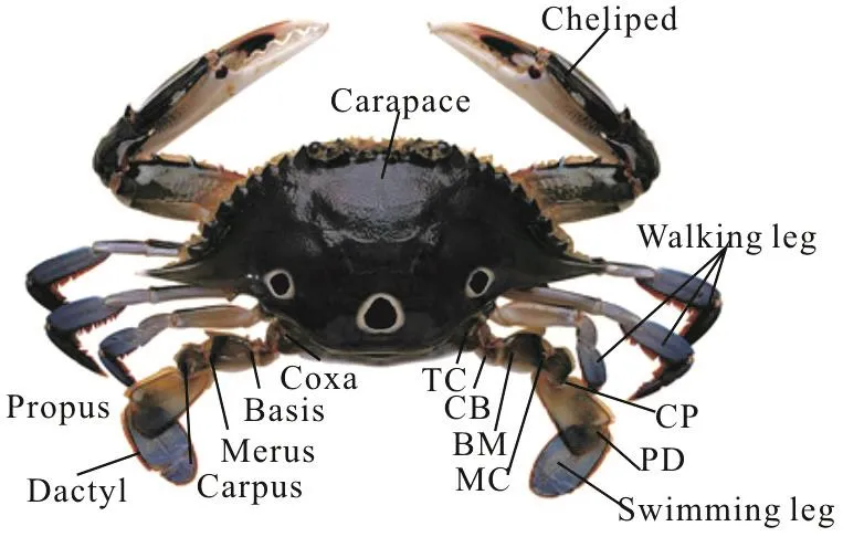
Fig. 1 (Color online) Shape structure of Portunus trituberculatus
The crab appendage consists typically of a shaft and 5 pereiopods. The Portunidae is characterized by the flattening of the last pair of legs to become swimming broad paddles, called the swimming legs.This ability, together with their strong chelipeds,allows many species to be fast and aggressive predators.

Fig. 2 (Color online) 3-D model of crab-like robot
The experimental study of the Portunidae by Vivo shows that the physiological structure of the swimming leg is similar to that of a walking leg. With the polyarticular skeleton texture, the swimming leg can achieve the flexible flapping under water. The typical swimming legs of the Portunidae consist of six components (the Coxa, the Basis, the Merus, the Carpus, the Propus, the Dacty1) articulated with each other by bicondylar joints[15]. The range of each segment motion is restricted to a single plane. Most of these planes are so positioned as perpendicular to the adjacent joints. 10 groups of stretched muscles are housed in the segments to control the movement of the swimming legs. The pleural muscles consist of 4 types,i.e., those of the Promotor, the Remotor, the Levator and the Depressor. The extensor and flexor musculature of the promotor, originated from the pleural venter and dorsum, generates the up-down motion of the Coxa around the TC joint. The mediolateral motion of the Basis around the CB joint is realized by the Levator and the Depressor. The flexer and extensor muscles in the Merus operate the MC joint to move the legs in the left-right direction. The stretcher and bender housed in the Carpus are responsible for rotating the Propus forward and backward. The opener and closer housed in the Propus operate the PD joint to move the Dacty1 in the up-down direction.Compared with the walking leg, the Propus and the Dacty1 of the swimming legs are muscular. Usually the Dacty1 is unfolded to achieve a greater thrust while the swimming leg is flapping. Both the ratio of the numbers of the nerve fibers and the ratio of the areas of the muscle fibers in the Propus and the Dacty1 are high.
2. Bionic structure design
2.1 Crablike robot prototype
Based on the bionic prototype of the Portunus trituberculatus, a new leg-paddle coupling crablike robot with the composite propulsion of walking legs and swimming legs and the capability of operating in shoals is designed, with the abilities of walking and swimming under water, as shown in Fig. 2.
The robot consists of three pairs of walking legs,a pair of swimming legs, embedded controller modules, a perception unit, a wireless communication part and an energy system. The joints of the crablike robot are driven by waterproof servos. The control system and the energy system are wrapped in a sealed cabin. The communication between the actuators and the control system is through the watertight connector arranged outside the sealed cabin.

Fig. 3 Coordinate system of the swimming leg
In view of the fact that the BM and CP joints with a small angle span during the flapping of the swimming legs can be neglected in the process of the design, a simplified swimming leg model is built, as shown in Fig. 3. Four waterproof servos are combined into an actuator to drive the hydrofoil. These servos are functioned to generate the feathering, lead-lag,flapping and rowing motions. The length of the swimming legs is 280 mm, and the proportions of the Coxa, the Basis, the Propus and the Dacty1 are 0.21,0.11, 0.43 and 0.25, respectively. The rotations of the TC, CB, BP and PD joints are controlled by the servos with angle spans of φTC(-90°≤φTC≤90°),φCB(-45°≤φCB≤90°), φBP(-90°≤φBP≤45°) and φPD(-30°≤φPD≤30°).
2.2 Kinematic model of swimming leg
Before analyzing the hydrodynamics of the swimming leg, a kinematic model of the swimming leg should be established. Then the mathematical relationships between the joint angles and the attack angles of the end-hydrofoil should be defined. Further,the joint trajectory plan should be made. In order to analyze the kinematic characteristics of the swimming leg, the inertial reference frame G- XYZ and the′ ′′′ for the Propus and the moving reference frame O-X Y Z moving reference frame O-X Y Z′′ ′′′′′′ for the Dactyl are defined accordingly as shown in Fig. 3.

Fig. 4 (Color online) Hydrodynamic experiment platform of swimmeret
The feathering angle, φTC, the lead-lag angle,, the flapping angle, φBP, and the rowing angle,, defined in Fig. 4, are sinusoidally varied:

where φTCA, φCBA, φBPAand φPDAdenote the amplitudes of the feathering motion, the lead-lag motion, the flapping motion and the rowing motion ,respectively. φTCC, φCBC, φBPCand φPDCare the biased angles of the feathering motion, the lead-lag motion, the flapping motion and the rowing motion,respectively. f and t denote the motion frequency of the swimming leg and the time. ΔφCBis the phase difference between the lead-lag motion and the feathering motion. ΔφBPis the phase difference between the flapping motion and the feathering motion. ΔφPDis the phase difference between the rowing motion and the feathering motion.
The asymmetric oscillations during the lead-lag motion and the flapping motion of the swimming legs are obtained through the real-time state monitoring and the data analysis of the marine crab movement. In general the down stroke motion takes less time than the upstroke motion. The lead motion takes less time than the lag motion. Due to the asymmetric motion,the effect of the added mass is enhanced and the aggregated vortex rope is merged into the hydrofoil trailing vortex, which increases the pressure and the strength of the jet in the wake. Consequently the thrust force is increased. A mathematical model of the pectoral fin oscillating in an asymmetric motion was set up by Su et al.[14]. The hydrodynamic performance of the pectoral-fin was analyzed when the asymmetric coefficient is 0.5. But in this model. a sudden change of the joint velocity cannot be realized in practice.These problems are solved by developing a new motion-time ratio model of the oscillating asymmetric motion of the swimming legs.

where subscript i stands for the TC joint, the CB joint, the BP joint and the PD joint, λ stands for asymmetric coefficients. In the drag-based swimming modeand in the lift-based swimming mode, where tF, tB, tUand tD,respectively, stand for the lead motion time, the lag motion time, the upstroke time and the down stroke time.
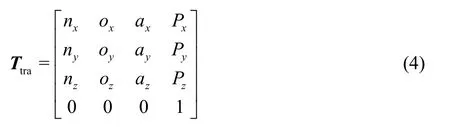
By the representation of the Denavit-Hartenberg for the robot manipulator, it is possible to define the homogeneous transformation matrices for adjacent links. The location of the end hydrofoil with respect to the inertial coordinate system is expressed as

And the homogeneous transformation matrices are
2.3 Hydrodynamic coefficient and efficiency of swimming legs
According to the above analysis and the coordinate system, the thrust force coefficient CX,the lateral force coefficient CY, the lift force coefficient CZ, the moment coefficient in XGdirection, the moment coefficient in YGdirection CMYand the moment coefficient in ZGdirection CMZare defined as follows:

The propulsive efficiency of a swimming leg,which is generally difficult to measure because of the large dynamic loads in both lift and thrust directions,is defined as the power output divided by the power input
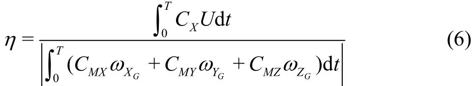

where


and α is the angle between the lateral axis of the inertial coordinate system and the lateral axis of the body coordinate system.
The Strouhal number related to the flapping hydrodynamic performance of the swimming leg[16]. It motion has an important influence on the is defined as

where b is considered here as the estimated length of the wake width, and U is the speed of the swimming leg.
The Reynolds number is expressed as[16]

where C is the chord length of the swimming leg and ν is the kinematic viscosity of the fluid.
3. Numerical calculation principle and method
3.1 Governing equations
The effects of the swimming leg oscillations on the fluid flow around such a body are highly unsteady,accompanied with different scale vortices, and a detailed analysis of the fluid-structure interactions is desirable. To simulate the time dependent unsteady viscous flow around an oscillating swimming leg, the unsteady Navier-Stokes equations with an incompressible assumption are used.
The governing equations for the unsteady incompressible flow are as follows:

where uidenotes the transient velocity component in i direction,and, respectively, represent the mean velocity components in i and j directions,ρ and μ are the density of the fluid and the dynamic viscosity,is the Reynolds shearing,is the source term,is the mean pressure. The modeled transport equations for k and ε in the practicable model are:
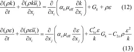
where Gkis the generation of k due to the mean velocity gradients,

3.2 Computational domain and grids
Because for the structured grid method, high quality grids are required, while the distortion of grids is magnificent when the bionic swimming leg is in movement. The precision of the computation using the structured grid method is not good enough. So in this paper the unstructured grid algorithm is used to guarantee the mesh quality near the swimming leg during its movement. In this method the grid zone is divided into two different domains. The interior domain created by the swimming leg and its near domain are moving together and the grid in them will be unchanged. The exterior domain, i.e., the domain between the outer edge of the inner domain and the far field is filled with unstructured grids, and the grid there will be changed to accommodate the swimming leg motion.
The spring based smoothing and Laplace local re-meshing method is applied to update the dynamic mesh during the motion of the flapping hydrofoil. To smooth the mesh, a value of 0.5 is used for the boundary node relaxation and a standard value of 0.001 is used for the convergence criterion and 0.01 for the Spring Constant Factor.
The main function of the 4th-DOF of the swimming legs is to expand and recover the hydrofoil,which mainly affects the value of the hydrodynamic coefficient more than its overall trend. This paper investigates the influence of the first three rotational degrees of freedom on the hydrodynamic performance of the swimming legs. The rigid hydrofoils of the swimming legs are simplified in the simulation and experiment, without the end degree of freedom.
4. Results and discussions
4.1 Hydrodynamic experiments
The major part of the hydrodynamic experimental platform is composed of the propulsion system, the control system and the hydrodynamic measurement system, as shown in Fig. 4. In the bionic swimming leg propulsion system, 4 waterproof servos HS-5646WP are used to control the joint movement. The hydrodynamic measurement system mainly consists of a 3-component force sensor, a CAN data acquisition card, and a dSPACE semi-physical simula- tion platform. The 3-axis piezoelectric force sensor is attached on the experimental platform to detect the lift,lateral and thrust forces, to be transferred to the dSPACE through the CAN bus. All signals are digitally filtered at 30 Hz before any calculation and plotting. The embedded control system based on the PC104 on the carriage controls the motions of the swimming legs through a servo motion control card.The hydrodynamic measurement platform is attached to a linear guide located above the free surface of water and can be translated at an adjustable velocity U. The hydrofoil of ABS material is made by the 3-D printing technique.
4.2 Hydrodynamics of swimming leg
In view of a close relationship between the reliability of the computation results using the CFD model and the quality of the mesh, in this section, the influence of the grid number in the computational domain on the computation accuracy is investigated.The thrust coefficient tends to be stable when the global grid numbers are over 3.1×10⁶. In this case, the calculation error is less than 1%, within the allowable range, as compared to the cases of 4.66×10⁶and 7.5×10⁶grid numbers. So, with 3.1×10⁶global grid numbers, the basic requirements for the 3-D numerical simulation can be met. More grid numbers may not improve the computation accuracy substantially withmore computation time.
In order to verify the numerical methods in this study, the computational results of both the blade element method[17]and the CFD method are compared with experimental results. The numerical computation and experiment conditions are: U=0.2 m/s ,φTCA=35°, φCBA=35°, φBPA=40°, ΔφCB=0°,ΔφBP=90°, f=0.5 Hz and Re=1.0× 10⁵, the unassigned parameters are set 0°, and the same is done in what follows.

Fig. 5 Comparison of hydrodynamic coefficients during one cycle: (a) Time record of the thrust coefficient in one cycle,(b) Time record of the lift coefficient in one cycle
Figure 5 shows the comparison of results of the FLUENT, the hydrodynamics experiment and the blade element method. It can be seen that the variation trends of the hydrodynamic coefficients of the two calculations are consistent with the experimental results. The extreme value and the inflection point are reached approximately at the same time, but with a certain gap, especially, for the peak value. There are three key factors related to the deviation between the experimental and numerical results. First, the experiment platform vibrates due to the movement of the swimming legs, which increases the interference between the swimming legs and the test platform.Second, the swimming legs are simplified as a rigid plate in the simulation. The motion of the actuator also generates some hydrodynamic force in the experiment besides the hydrofoil, i.e., the surface area of the hydrofoil increases. Third, compared with the viscosity model in the CFD method, the fluid separation and turbulence model in the experiment is more complex.
4.3 Trail vortex structure
The 3-D vortex contours of the swimming leg in a cycle are shown in Fig. 6.

Fig. 6 (Color online) Vortices in an motion period

Fig. 7 (Color online) The distribution of shedding vortices
Due to the complexity of the 3-D vortex structure,this paper employs the slice method to analyze the trail vortex of the swimming legs. Figure 7 shows the contours of the vorticity ξyin the direction of Y-axis on the section of Y=100 mm , which depicts the consumption and the shedding of the trail vortex.There are two pairs of vortices on the top and the bottom, which shed sequentially in a motion period.Around 1/4T, an anti-clockwise vortex (ξy>0)and a clockwise vortex (ξy<0) shed below the swimming leg hydrofoil. Around 3/4T, an anticlockwise vortex (ξy>0) and a clockwise vortex(ξy<0) shed below the hydrofoil. By the comparison of the contour structure of the 2-D and 3-D airfoil in the case of flapping, there is a single-row reverse Karman Vortex Street in the wake of the 2-D airfoil edge, while a double-row vortex pair appears in the wake of the 3-D airfoil edge, which significantly improves the propulsion of the hydrofoil[18].
4.4 Hydrodynamic performance of 2DOF swimming leg
4.4.1 Effect of phase difference on hydrodynamic performance
In this part, the effect of the phase difference between the feathering and flapping motions on the swimming leg hydrodynamics is studied by experimental and CFD methods. The motion parameters are as follows: U =0.2 m/s , φTCA=35°,φCBA=40°, f=0.5 Hz and ΔφBP=-120°-120°.
Figure 8 shows the time variation of the hydrodynamic coefficient CXfor various phase differences ΔφBPbetween the feathering and flapping motions. It is seen that during one flapping period, the variation trends of the hydrodynamic coefficient CXare almost the same for different values of ΔφBP. There are two peak values, with the first peak value at 1/2T and the second peak value at the end of the cycle. We can further find that the change of ΔφBP, results in not only a change of the magnitude of the peak value of the thrust coefficient CX, but also a change of the time when the peak value occurs Meanwhile, the value of the thrust coefficient CXdecreases and the time when the peak value occurs are increased if ΔφBPincreases.
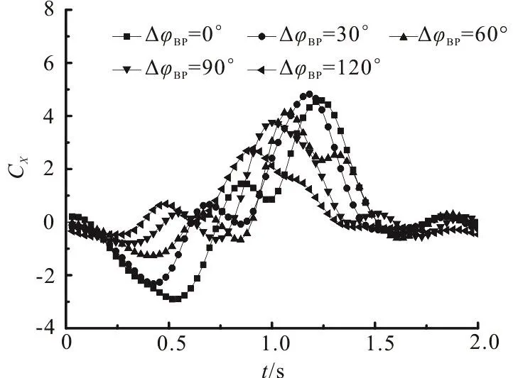
Fig. 8 Hydrodynamic coefficients with various ΔφBP obtained by experimental method
Figure 9 shows the curves of the average thrust coefficient CXmand the propulsive η against the phase difference ΔφBPfor the flapping frequency f equal to 0.5 Hz, 1.0 Hz and 1.5 Hz. From Fig. 9 we can see that with the increase of f, the range of the phase difference ΔφBPfor CXm≥0 extends. The average thrust coefficient (CXm≥0) reaches the maximum between the phase differences of 90° and 120° and the maximum value increases as the flapping frequency f increases. When the flapping frequency f keeps constant, the average propulsive efficiency η first rises and then decreases with the increase of ΔφBP. The maxima of the efficiency η at a fixed frequency f can be distinguished for f=0.5 Hz,1.0 Hz and 1.5 Hz, they, respectively, occur at the values of ΔφBPequal to 90°, 120°. The peak value of the efficiency η decreases with f.

Fig. 9 Influence of ΔφBP on hydrodynamic performance obtained with the numerical method
4.4.2 Effects of Strouhal number and flapping amplitude on hydrodynamic performance
The motion parameters of the swimming leg are set as follows: φTCC=0°, φCPC=0°, φTCA=35°and φBPA=10°, 20°, 30° and 40°. The experimental values of the average thrust coefficient CXmand the propulsive efficiency η are plotted as the functions of the Strouhal number St in Figs. 10, 11. Figure 10 shows that the variation trends of the average thrust coefficient CXmversus the Strouhal number St for various φBPAare similar. The average thrust coefficient CXmmonotonically increases with St.Increasing St, one sees a continuous change from a drag-producing motion (CXm<0) to a thrustproducing motion (CXm>0). When St>0.2, the positive average thrust coefficient CXmcan be obtained. The maximum average thrust coefficient CXmis reached when St comes to 1.0, which will benefit the propulsion of the swimming leg. With the same St , when the flapping amplitude φBPAincreasesfrom φBPA=10° to φBPA=40°,CXmdecreases.
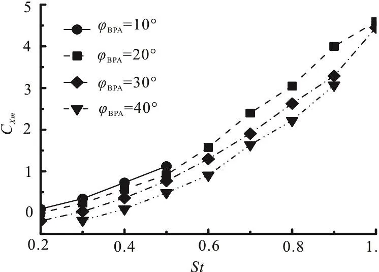
Fig. 10 Influence of St on thrust coefficient obtained with numerical method

Fig. 11 Influence of St on propulsive efficiency obtained with numerical method
Figure 11 shows that with various φBPA, on the curves of the efficiency η vs. the Strouhal number St , a maximum efficiency η is observed with Stmaxbeing between 0.3 and 0.5. According to the analysis of the fish swimming body and posterior fin mode by Triantafyllou et al.[19], St is between 0.2 and 0.4.According to Taylor et al.[20], for birdʼs wing in the flapping mode, its efficiency reaches the maximum when St is equal to a value in the range of 0.3-0.5, as in a good agreement with the St range of the swimming leg with a high efficiency. When St is increased, the efficiency η increases quickly until it reaches Stmax, then η decreases if St continues to increase. The maximum efficiency η is 53.52%when φCPA=10° and St=0.3. The corresponding average thrust coefficient CXmis very small and as small as 0.35. Through the above analysis, we can see that when the value of St is slightly larger than Stmax, a relatively high efficiency together with a high average thrust can be achieved. In the range of small values of φBPA, the efficiency η is high, but it decreases when φBPAis increased from 10° to 40°.
The experimental results of the thrust coefficient CXversus time for various flapping amplitudes φBPAare as shown as in Fig. 12. It can be seen that the variation trends of CXwith various φBPAare similar. The time at which the peak value occurs is approximately the same but the magnitude of the peak value will increase if φBPAincreases.

Fig. 12 Hydrodynamic coefficients for different φBPA obtained with experimental method
4.4.3 Effect of flapping biased angle on hydrodynamic performance
The parameters for the numerical simulation and the experiment are: φTCC=φCPC=0°, φTCA=35°,φBPA=40°, f=0.5 Hz, the value of the flapping biased angle φBPCis equal to 5°, 10°, 15° and 20°.
Variations of the average thrust coefficient CXmand the average lift coefficient CZmare plotted in Fig.13, when the flapping biased angle φBPCvaries from 0° to 40°, St is equal to 0.8 and 1.0, respectively,where the horizontal axis represents CXmand the vertical axis is CZm.
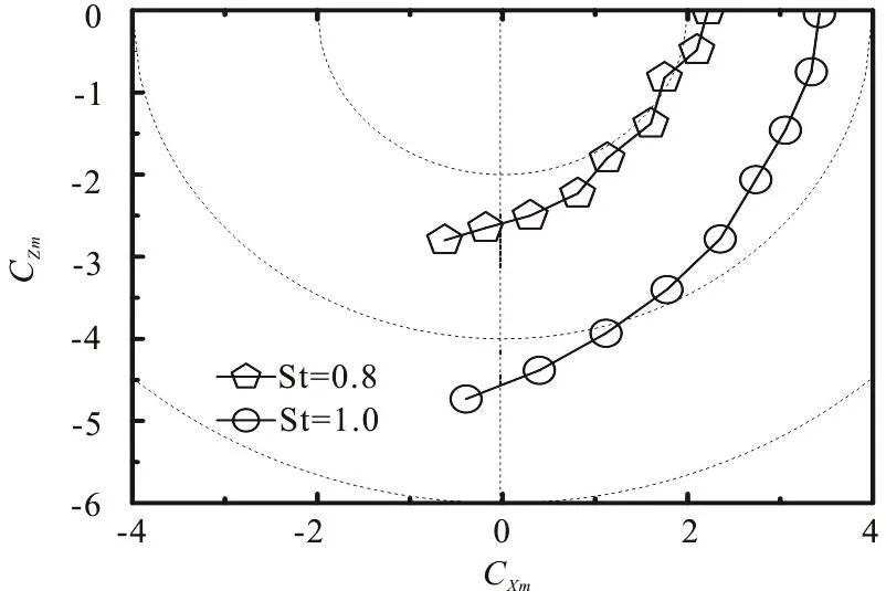
Fig. 13 Influence of φBPC on hydrodynamic performance obtained with numerical method
We can see that with a small flapping biased angle φBPC, the lift force has an asymmetrical distributions in positive and negative regions.Approximately a zero average lift force can be obtained when the biased angle is zero. Applying a flapping biased angle will considerably increase the average lift coefficient CZm. The average thrust coefficient CXmdecreases with the increase of φBPC,and negative values of CXmare obtained, when φBPC≥33.4° for St=0.8 and φBPC≥37.8° for St=1.0. Hence, it is indicated that a high St will increase the thrust.
4.4.4 Effect of feathering amplitude on hydrodynamic performance
The parameters for the numerical simulation and the experiment are: φTCC=φCPC=0°, φBPA=40°,ΔφBP=90°, f=0.5 Hz and the feathering amplitude φTCAis equal to 10°, 20°, 30° and 40°, respectively.
Numerical results of the average force coefficient and the propulsive efficiency are plotted as the functions of the feathering amplitude as shown in Fig.14. We can see that when φTCAis increased, the absolute values of CXm, CYmand CZmall increase but in different rates. The rate of CYmis the maximum, the rate of CZmis the minimum. The propulsive efficiency monotonously increases with the increase of φTCAfrom 0° to 40°.
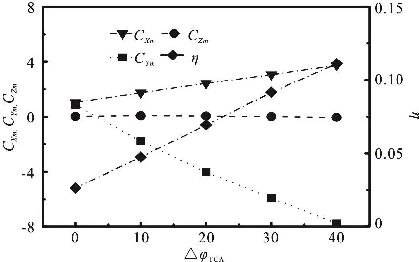
Fig. 14 Influence of φTCA on hydrodynamic performance obtained with numerical method
4.4.5 Effect of flow velocity on hydrodynamic performance
The operating conditions are: φTCC=φCPC=0°,φTCA=35°, φBPA=40°, ΔφBP=90°, f=1.0 Hz,the flow velocity increases from 0.1 m/s to 0.6 m/s with an increment of 0.1 m/s.

Fig. 15 Influence of U on hydrodynamic performance obtained with numerical method
Figure 15 shows that the average thrust and lateral force coefficients (absolute values) sharply decrease with the increase of the flow velocity when the flow velocity is less than 0.3 m/s. A very slight decrease of the thrust and lateral force coefficients(absolute values) can be seen when the flow velocity increases further in the large velocity range (0.3 m/s-0.6 m/s). The average lift coefficient approaches zero and remains constant with the increase of the flow velocity. Figure 18 shows that the propulsive efficiency increases with the increase of the flow velocity when the flow velocity is less than 0.3 m/s.After the maximum propulsive efficiency of 42.2% is achieved at U =0.3m/s , it starts to decrease until it is zero, where the average thrust coefficient is very small. Thus the flow velocity 0.2 m/s is selected in the next numerical calculation and experiment.
4.5 Hydrodynamic performance of 3DOF swimming leg
In this part the hydrodynamic performance of the 3DOF swimming leg is studied. The leg motion relative to the body consists of feathering, lead-lag and flapping motions.
4.5.1 Effect of phase difference on hydrodynamic performance
Figure 16 shows the average hydrodynamic coefficient and the propulsive efficiency against ΔφCBfrom -120° to 120° with various flapping frequencies f and the other parameters, φTCC=φCBC=φBPC=0°, φTCA=35°, φCBC=30°, φBPA=40°, ΔφBP=90°, U=0.2 m/s.
We can see a slight change of the average hydrodynamic coefficient. The maximum value of CXm, is obtained when ΔφCB=0°. With the increase of ΔφCBin the range -120°≤ΔφCB≤-90°, the propulsive efficiency gradually decreases. The mini-mum propulsive efficiency is obtained at ΔφCB=-90°. With the increase of ΔφCBin the range-90°≤ΔφCB≤0° the propulsive efficiency gradually increases. The highest value of the propulsive efficiency is obtained at ΔφCB=0° and after that it decreases. Comparing the curves of the propulsive efficiency with 3 different frequencies, we can see that with a low flapping frequency (0.5 Hz), the propulsive efficiency is low and with the medium frequency(1.0 Hz), the propulsive efficiency is maximized. A higher frequency (1.5 Hz) will decrease the propulsive efficiency again. A maximum efficiency of around 34%is achieved at f=0.5 Hz and ΔφCB=0°. Comparing with the result from the hydrodynamic experiment of the 2DOF swimming leg, it is shown that adding the lead-lag motion (3DOF) cannot increase the thrust significantly and cannot decrease the propulsive efficiency distinctly either.

Fig. 16 Influence of ΔφCB on hydrodynamic performance obtained with numerical method
4.5.2 Effect of lead-lag biased angle on hydrodynamic performance
Parameters for the numerical simulation and experiment are: φTCC=φBPC=0°, φTCA=35°,φCBA=30°, φBPA=40°, ΔφBP=90°, ΔφCB=0°,U=0.2 m/s , f=0.5 Hz and the range of the lead-lag biased angle is φCBC=10°-30°.
Figure 17 shows the average hydrodynamic coefficient and propulsive efficiency as functions of the lead-lag biased angle for the swimming leg. The average lift and lateral force coefficients are proportional to the lead-lag biased angle between 0°and 40°. Increasing the lead-lag biased angle φCBC,we also observe that the average thrust coefficient first increases and then decreases. The maximum average thrust coefficient is CXm=5.95 at φCBC=30°. The curve of the pr opu lsive eff icienc y has the same variation trend astheaveragethrustcoefficient.The peak propulsive efficiency occurs at φCBC=20°.

Fig. 17 Influence of φCBC on hydrodynamic performance obtained with numerical method
4.5.3 Effect of lead-lag amplitude on hydrodynamic performance
Figure 18 shows the average hydrodynamic coefficient and propulsive efficiency versus φCBAfor φTCC=φCBC=φBPC=0°, φTCA=35°, φBPC=40°,ΔφBP=90°, ΔφCB=0°, U =2.0 m/s , f=1.0 Hz .

Fig. 18 Influence of φCBA on hydrodynamic performance obtained with numerical method
As φCBAincreases from 0° to 40°, the variances of CXmand CYmare very small and the absolute value of CZmincreases considerably. The propulsive efficiency, η, quickly decreases at the beginning(0°<φCBA<5°) until it becomes negative and then decreases gently.
4.5.4 Effect of foil thickness on hydrodynamic performance
In order to investigate the influence of the foil thickness on the hydrodynamic performance, three thicknesses (1.5 mm, 3.0 mm and 4.5 mm) are considered in the experiment. The experimental results are as shown as in Figs. 19, 20. When the flapping frequency is 0.5 Hz, the average thrust coefficient is very small for all foil thicknesses. How- ever, when the flapping frequency is high (1.5 Hz), a thin foil(1.5 mm) results in a high thrust coefficient (9.0) and a thick foil (4.5 mm) results in a low thrust coefficient(7.5).
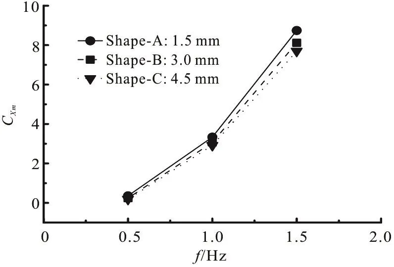
Fig. 19 Influence of foil thickness on hydrodynamic coefficients obtained with numerical method
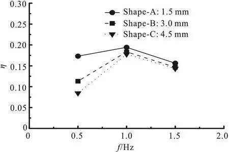
Fig. 20 Influence of foil thickness on propulsive efficiency obtained with numerical method
Figure 20 shows that the propulsive efficiency decreases with the increase of the foil thickness at a low frequency (0.5 Hz). But the foil thickness has a small effect on the propulsive efficiency when the flapping frequency is high (1.5 Hz). The maximum propulsive efficiency of 19.8% is achieved at f=1.0 Hz when the foil thickness is 1.5 mm. The results suggest that the crab-like robot can swim faster and more efficiently with a thin foil (1.5 mm) than a thick one (4.5 mm).
5. Conclusions
In this study, a leg-paddle coupling crablike robot is developed. The hydrodynamic performance of the swimming leg is studied with numerical simulations and experiments. The effects of kinematic parameters and foil thickness on the hydrodynamic performance are also discussed. The following conclusions are drawn:
(1) The numerical simulation and experiment for the oscillating foil of a swimming leg provide systematic data on thrust, lateral and lift forces generated harmonically. The propulsion tests show the optimum thrust and propulsive efficiency for a certain combination of parameters like the phase difference,the flapping amplitude, the biased angle of the coupling movement and the Strouhal number.
(2) The double-row vortex pair appears during the flapping motion of the hydrofoil, which significantly improves the propulsion of the hydrofoil.
(3) The foil thickness has effects on the hydrodynamic performance of the swimming leg. Large thrust and high efficiency can be obtained by a thin foil (1.5 mm).
猜你喜欢
Chinese Physics B(2022年8期)2022-08-31
天工(2021年2期)2021-03-03
小哥白尼(野生动物)(2019年4期)2019-09-10
数学学习与研究(2017年2期)2017-03-06
校园英语·下旬(2016年2期)2016-03-18
小学阅读指南·高年级版(2015年2期)2015-09-10
中国新时代(2012年1期)2012-02-19
意林(2010年11期)2010-05-14
故事林(2007年2期)2007-05-14

- 水动力学研究与进展 B辑的其它文章
- Call For Papers The 3rd International Symposium of Cavitation and Multiphase Flow(ISCM 2019)
- A well-balanced positivity preserving two-dimensional shallow flow model with wetting and drying fronts over irregular topography *
- Determination of epsilon for Omega vortex identification method *
- Transient curvilinear-coordinate based fully nonlinear model for wave propagation and interactions with curved boundaries *
- Tracer advection in a pair of adjacent side-wall cavities, and in a rectangular channel containing two groynes in series *
- Numerical simulation of transient turbulent cavitating flows with special emphasis on shock wave dynamics considering the water/vapor compressibility *