
A well-balanced positivity preserving two-dimensional shallow flow model with wetting and drying fronts over irregular topography *
2018-09-28 05:34GangfengWu吴钢锋ZhiguoHe贺治国LiangZhao赵亮GuohuaLiu刘国华
水动力学研究与进展 B辑 2018年4期
Gang-feng Wu (吴钢锋), Zhi-guo He (贺治国), Liang Zhao (赵亮), Guo-hua Liu (刘国华)
1. School of Civil Engineering and Architecture, Ningbo Institute of Technology, Zhejiang University, Ningbo 315100, China
2. Institute of Port, Coastal and Offshore Engineering, Ocean College, Zhejiang University, Hangzhou 310058,China
3. Institute of Hydraulic Structures and Water Environment, Zhejiang University, Hangzhou 310058, China
Abstract: This paper presents an improved well-balanced Godunov-type 2-D finite volume model with structured grids to simulate shallow flows with wetting and drying fronts over an irregular topography. The intercell flux is computed using a central upwind scheme, which is a Riemann-problem-solver-free method for hyperbolic conservation laws. The nonnegative reconstruction method for the water depth is implemented to resolve the stationary or wet/dry fronts. The bed slope source term is discretized using a central difference method to capture the static flow state over the irregular topography. Second-order accuracy in space is achieved by using the slope limited linear reconstruction method. With the proposed method, the model can avoid the partially wetting/drying cell problem and maintain the mass conservation. The proposed model is tested and verified against three theoretical benchmark tests and two experimental dam break flows. Further, the model is applied to predict the maximum water level and the flood arrival time at different gauge points for the Malpasset dam break event. The predictions agree well with the numerical results and the measurement data published in literature, which demonstrates that with the present model, a well-balanced state can be achieved and the water depth can be nonnegative when the Courant number is kept less than 0.25.
Key words: Shallow water equations, central upwind scheme, well-balanced, wetting and drying, positivity preserving, second order accuracy
Introduction
The 2-D shallow water equations (SWEs),obtained by integrating the Reynolds-averaged Navier-Stokes equations over the water depth, are widely applied to mathematically describe the free surface water flows over an irregular topography (e.g.,urban floods resulting from dam breach[1-2], heavy rainfall and tsunami, long wave runup; estuarine and coastal circulation). Because analytical solutions of the SWEs are only available for very few simple and ideal situations, it is important to develop robust and accurate numerical methods to solve the SWEs in more realistic engineering applications.
Various numerical methods were developed for the solutions of the shallow water systems, such as the finite difference methods[3-4], the finite element methods[5]and the finite volume methods[6-7]. With the finite volume methods, the shallow water equations are solved in the integral form in the computational meshes. Therefore, the mass and the momentum are conserved in each cell, even in the presence of flow discontinuities, which makes the finite volume techniques more efficient and robust. In recent years,the Godunov-type finite volume schemes were extensively applied to numerically solve the SWEs[8-10].The performance of these schemes was greatly improved in accuracy, stability, and shock-capturing ability.However, there are still some challenges when solving the SWEs by using the finite volume method with fixed grids.
One of the main difficulties is in constructing a numerical scheme to preserves the steady state at the discrete level. A numerical scheme is considered to be well-balanced or satisfying the C-property if it exactly preserves the “lake at rest” steady-state solution. If the traditional numerical schemes are not well-balanced, a spurious oscillation will be generated around the steady state, as so-called the numerical storm. In order to correctly represent the steady state, the grid must be extremely refined, making the algorithm highly inefficient. Therefore, the development of wellbalanced schemes becomes an important issue and some well-balanced methods were successfully developed[10-14]. Zhou et al.[12]adopted the surface gradient method, to reconstruct the water surface level instead of the water depth, to preserve the static condition on the structured grids. Based on those methods, Liang and Borthwick[13]and Duran et al.[14]further developed a mathematical balancing method to solve the pre-balanced SWEs, with good results with both structured and unstructured meshes. The key point of all these methods is to treat the slope source term in a manner to ensure the cancelation of the flux difference under the stationary flow condition and thus, the scheme is made to be well-balanced or to satisfy the C-property.
Another difficulty arising when numerically solving the SWEs with a fixed grid finite volume scheme is to simulate the wetting and the drying fronts.In the finite volume schemes, the flow velocity is calculated by dividing the unit discharge by the water depth, resulting sometimes in unphysical high velocities at the rapidly moving wet/dry fronts. Thus, the water depth might become negative, and the numerical calculation will break down. Many finite volume models were proposed to preserve the positivity of the water depth at the wet/dry fronts[15-19].However, only few of them[16-17,19]satisfy at the same time the well-balanced property. In addition, near the wet/dry front, where the water depth nearly vanishes,the friction term will cause a stiff problem, to significantly affect the stability of the numerical calculation. Therefore, in order to enhance the stability of the numerical solution near the dry area, it is necessary to keep the water depth positive at all time with a robust scheme, such as a semi-implicit scheme, for the friction term in modeling the water flows over an irregular terrain.
Recently the Godunov-type central upwind scheme was proposed by Kurganov and Levy[18], as a universal Riemann-problem-solver-free method for hyperbolic conservation laws, and it attracted much attention due to its simplicity, robustness and efficiency. Kurganov and Petrova[17]used the central upwind scheme to solve the 1-D and 2-D shallow water system numerically with a discontinuous bottom topography. Due to the fact that the friction terms are ignored in their model, it cannot be used in practical applications directly. Singh et al.[19]developed a 2-D shallow flow model for practical dam-break simulations by using the Godunov-type central upwind scheme, with satisfactory simulation results. However,when the dry area is contained in the computational domain, this model cannot preserve the “lake at rest”steady state unless the computational grid is adjusted at the wet/dry fronts[20]. The reason can be explained by using Fig. 1. When the bed elevation is defined at the cell corner and the flow variables are defined at the cell center, we might have partially wetted cells near the wet/dry fronts as shown in Fig. 1(a). In order to handle the partially wetted cells, the slope of the water surface is simply altered in the model as shown in Fig. 1(b) to ensure the partially wetted cells to be transformed into fully wetted ones. Obviously, this treatment violates the well balanced property of the numerical model.

Fig. 1 (Color online) Stationary state with dry boundaries
Therefore, this paper proposes an improved 2-D shallow water numerical model to deal with the aforementioned problems. The proposed model follows the Godunov-type central upwind scheme but improves the treatment of the wet/dry front for the shallow flow over the irregular topography.
1. Numerical model
1.1 Governing equations
The 2-D shallow water equations in the conservative form, obtained by integrating the 3-D Navier-Stokes equations over the water depth, are written in a vector form as:


where q, f, g and S are, respectively, the vectors representing the conserved flow variables, the fluxes in x and y directions and the source terms,t indicates the time, x and y are the Cartesian coordinates, η is the water surface elevation, zbis the bed elevation over the datum, h is the water depth. As shown in Fig. 2, the water depth can be expressed as h=η-zb. u and v are the depthaveraged velocity components in x and y directions, respectively, g is the gravitational acceleration, n is the Manning coefficient. One of main reasons for using the conservative form of the SWEs is that the resulting numerical models behave better than the primitive form in modeling the flows with shock, such as the dam break flows[21].

Fig. 2 (Color online) Sketch of water surface elevation, water depth, and bed elevation
1.2 Numerical scheme
The conservative shallow water equations (1) and(2) are discretized spatially with the structured grids using a finite volume Godunov-type approach, and the central upwind scheme is used to solve the flux at the volume interface. The slope limited linear reconstruction method is adopted to achieve the second-order accuracy in space. The method of the nonnegative reconstruction of the water depth proposed by Liang[15]is incorporated into the present model for the treatment of the wetting and drying fronts.
1.2.1 Discretization using finite volume method
The discretization of Eq. (1) is based on the finite volume method. As shown in Fig. 3, the non-staggered structure grids are adopted, in which the conserved variables and the bottom bed elevation are defined at the cell center and represent the average values of each cell.
Integrating Eq. (1) over the cell i, j and applying the Greenʼs theorem, we have
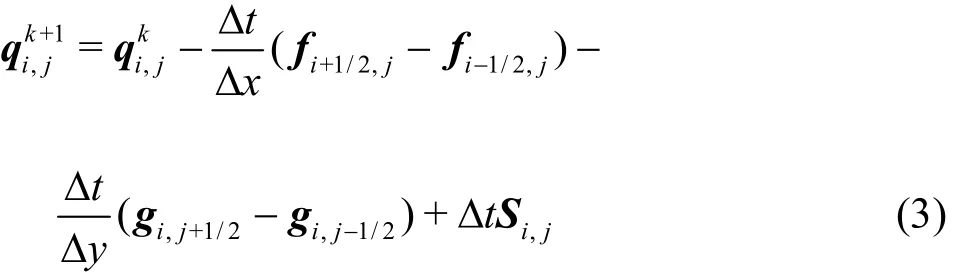
where the superscript k is the time level, the subscripts i and j are indices of the cell, Δt, Δx and Δy are the time step, and the cell sizes in x and y directions, respectively. fi+1/2,j, fi-1/2,j, gi,j-1/2and gi,j+1/2are the flux at the interface of the cell i, j. Si,jrepresents the source terms evaluated at the cell center. In Eq. (3), the time-marching method is used with the first-order accuracy in time to update the flow variables for a new time step. The second-order accuracy in time can be achieved using a Runge-Kutta method. However, in this paper, the time integration is carried out using the first-order Eulerʼs method.
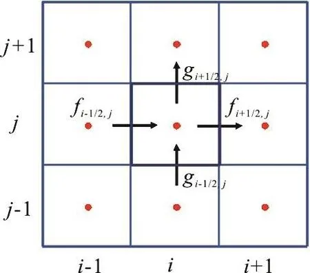
Fig. 3 (Color online) Definition of a cell centered grid
1.2.2 Nonnegative reconstruction of Riemann states
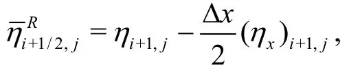
In the present Godunov-type framework, the interface fluxes are calculated using a central upwind scheme, which requires a correct reconstruction of the Riemann states at the interface. The method of the nonnegative reconstruction of the water depth method proposed by Liang[15]is shown to be accurate to deal with the wetting and drying fronts. Therefore, this method is applied to calculate the Riemann states. The Riemann states, the flow variables defined at the interface, are obtained from the available flow infor-mation at the cell center by using a slope limited linear reconstruction. For instance, the left face values at the cell interface (i+1/2,j) are given by:
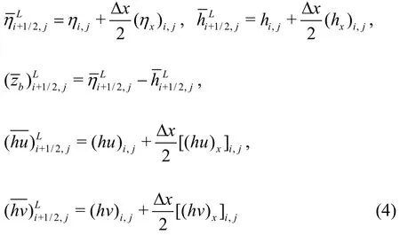
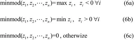
where (ηx)i,j, (hx)i,j, [(hu)x]i,jand [(hv)x]i,jrepresent the numerical derivatives of the flow variables in the cell (i, j). In order to preserve the stability of the model, one-parameter family of the generalized minmod limiters are used to calculate the numerical derivatives. Taking (ηx)i,jas an example

where θ is the parameter to control the numerical viscosity. In general, a larger value of θ makes the numerical results less dissipative and more oscillatory.θ=1.3, as suggested by Kurganov and Petrova[17]is adopted in this study. The minmod function is defined as
The values of (hx)i,j, [(hu)x]i,j, and [(hv)x]i,jcan be obtained in a similar way.
Similarly, the right face value of the cell interface(i+1/2,j) can be calculated by:

In order to obtain the final Riemann states,Audusse et al.[16]suggested that the bed elevation should be a single value and defined as

Then, the face values of the water depth are redefined as

Obviously, this method ensures that the reconstructed water depth is nonnegative. However, the reconstructed water depth may be very small or zero, which leads to large values of the flow velocity, making the model unstable. In order to prevent this happening, the regularization technique suggested by Kurganov and Petrova[17]is used to calculate the corresponding velocity components of the interface:
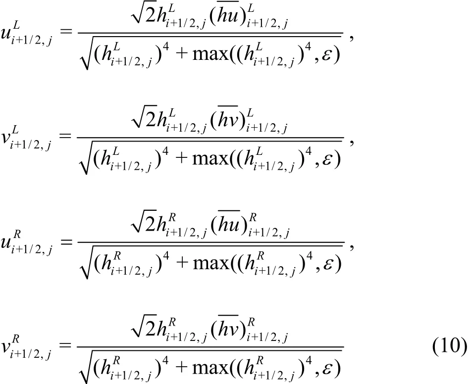
where ε is an empirically pre-defined positive number with ε being 10-6m in all simulations in this paper. It should also be mentioned that ε=10-6m is used to distinguish the dry and wet cells. When the water depth at the cell center is less than 10-6m, the cell is defined as a dry cell and the velocity is set to be zero without solving the momentum equations.
Hence, the Riemann states of other flow variables can be recalculated by:

For wet-bed applications, the above procedure obviously does not affect the well-balanced property of the numerical scheme. However, the local bed modifications are needed to obtain the well-balanced solution for a dry-bed application. As shown in Fig. 4, a wet cell (i, j) shares the common edge (i+1/2,j) with the dry cell (i+1,j), and the bed elevation of the dry cell is higher than the water surface elevation in cell(i, j). The stationary water at the static state is considered with u=0, v=0 and η=constant at the wet area. After the aforementioned reconstruction at the cell interface (i+1/2,j), the components of the Riemann states are given by:

Therefore, the fluxes at the cell interface (i+1/2,j)are calculated using the bed elevation (zb)i+1/2,jrather than the actual water surface elevation η of the cell (i, j). However, the fluxes at the cell interface (i-1/2,j) are estimated using the actual water surface elevation η of the cell (i, j), with a net flux in the cell (i, j), which violates the well-balanced property of the scheme. The local bed modification is implemented to overcome this difficulty by Liang[15].As shown in Fig. 4, the difference between the actual and reconstructed water surfaces at the interface(i+1/2,j) is calculated by:

Subtracting Δz from the original reconstructed value,the bed elevation and the water surface are given by:


Fig. 4 (Color online) Local bed modification for dry-bed application
1.2.3 Central upwind scheme
Many schemes were proposed to calculate the flux at the cell interface in recent twenty years. The Godunov-type central upwind scheme proposed by Kurganov and Levy[18]is adopted in this study since this scheme does not require solving the Riemann problems, and has been successfully used in shallow water flows over irregular terrains[19]. The major advantages of the Godunov-type central upwind scheme are the efficiency, the simplicity, and the robustness, which make this scheme very suitable for the shallow water model. Therefore, the flux of the central upwind scheme can be calculated by:

where fLand fRare the flux vectors in x direction on the left and right hand sides of the cell interface (i+1/2, j), respectively.,are the reconstructed Riemann states on the left and right hand sides of the cell interface (i+1/2, j), respectively.gLand gRare the flux vectors in y direction on the left and right hand sides of the cell interface(i, j+1/2), respectively.,represent the reconstructed Riemann states on the left and right hand sides of the cell interface (i, j+1/2), respectively.are the one-sided local wave speeds in x and y directions, respectively, and can be calculated as:

1.2.4 Discretization of the source term
The source term, as shown in Eq. (2), can be split into the bed slope terms and the friction terms. It is important to discretize the bed slope terms appropriately to ensure the scheme to be well balanced.Hence, the bed slope terms are approximated as follows:

Herein the bed elevations are a single value, which is modified by Eq. (14).
In general, a simple explicit discretization of the friction term may cause numerical instability when the water depth is very small. To overcome this difficulty,the implicit treatments[8]and the semi-implicit treatments[7]are widely used. In this study, the friction terms are discretized by using the semi-implicit treatment[7]which is given by:

where the superscript k represents a time level. Substituting Eq. (23) and Eq. (24) into the time marching Eq. (3), the values of the flow variables at the end of the time step can be obtained.
1.2.5 Stability criteria and boundary conditions
The current numerical scheme is explicit and its stability is governed by the Courant-Friedrichs-Lewy(CFL) criterion. In order to preserve the positivity of the water depth at each time step, the Courant number has to be kept less than 0.25[17]. Therefore, the CFL restriction for the current model is

where NCFLrepresents the Courant number, and a and b are given by:

Generally, two kinds of boundaries, i.e., the open boundary and the wall boundary, are encountered in the numerical model. For the open boundary, the flow variables in the ghost cells are usually determined by solving a boundary Riemann problem, as is related to the local flow regime. For the wall boundary, the velocity normal to the boundary and the water surface gradient are both set to be zero at the boundary, as shown to be second-order accurate[22].
2. Numerical results
In this section, three theoretical benchmark tests,two laboratory dam break flow experiments, and a real dam failure event are simulated to test the performance of the proposed model. For all tests, g=9.81m/s2and ρ=1000 kg/m3.
2.1 Test for well-balanced property
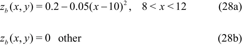
The first test is to check the current modelʼs ability of simulating the stationary steady flow with the wet/dry interface over an uneven bed. A bump is located at the center of a 1 m×1 m channel, with the bed elevation defined by[21]

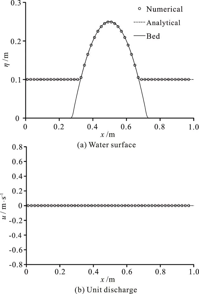
Fig. 5 The simulated results along the line of y=0.5m at t=100s with our model
The channel is frictionless and all four sides are closed by the vertical wall. As the initial condition, the water in the channel is stationary, with the water surface elevation being defined asSo the bump at the center of the channel is partially submerged. The steady state should be exactly preserved by the numerical models. The total simulation takes 100 s, using 50×50 cells with a uniform cell size of 0.02 m. The time step is determined by the CFL criteria. Figures 5, 6 show the simulated results of the water surface and the unit discharge along the line of y=0.5 mat t=100s by our model and by the model developed by Kurganov and Petrova[17]. The results show that the water surface remains unchanged and no unphysical discharges are found in the results obtained with our model, which verifies the well balanced property of the proposed model. Howerver,unphysical discharges are found in the results obtained with the model developed by Kurganov and Petrova[17], which violates the well balanced property.

Fig. 6 The simulated results along the line of y=0.5m at t=100s with the model developed by Kurganov and Petrova[17]
2.2 1-D steady flow over a bump
The benchmark test of a 1-D steady flow over a bump is to check the convergence ability and the accuracy of the model. The flow occurs in a 25 m×1 m frictionless channel with the bed defined as:
According to the initial and boundary conditions,the steady flow over the bump can be supercritical,transcritical with or without shock, or subcritical.Herein, the subcritical flow case, which is the most challenging to the numerical model[13], is chosen to test the modelʼs convergence ability and the order of accuracy. In the case of a steady subcritical flow, a unit discharge of 4.42 m2/s is imposed at the upstream boundary and a fixed water depth of 2.0 m at the downstream boundary. The initial water surface elevation and the unit discharge in x direction are set to be 2.0 m and 4.42 m2/s at each cell, respectively.The model is run 400 s to ensure that the steady state is reached. In order to evaluate the convergence of the grids, four different grids with the mesh sizes of Δx=0.05 m, 0.10 m, 0.13 m and 0.25 m are considered in this study. Table 1 compares the L1and L2error norms of η and q as a function of the grid size Δx which are defined as:

where N is the total number of the computational cells,iaη and qiadenote the analytical solutions that are derived by using the Bernoulliʼs theorem. It can be concluded from Table 1 that the model is sufficiently accurate and the deviation between the numerical and analytical results of the unit discharge is larger than the water level, which is also reported in Song et al.[21]. L2error norms of η and q are presented in Fig. 7. The plot shows that L2error norms vanishes as2()OΔx when the grid is progressively refined.

Table 1 L1 and L2 error norms in η and q as a function of grid size Δx
2.3 Oscillatory flow in a parabolic bowl
In order to verify the capability of the proposed model for accurately simulating the wetting and drying fronts over the an uneven topography, the oscillatory flow in the parabolic bowl is investigated in this study[23]. The oscillatory flow is assumed to take place in a parabolic bowl with the bed elevation described as


Fig. 7 L2 error norms of η and q as function of Δx
where h0and a are positive constants. The analytical solution of the 2-D frictional flow is given by Wang et al.[23]
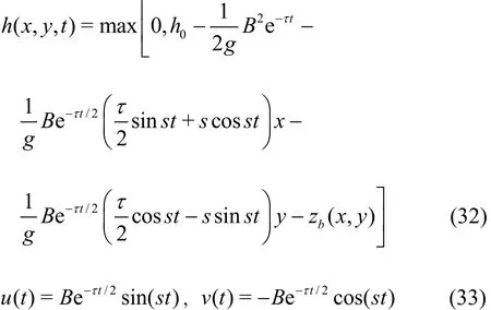
where τ denotes the bed friction parameter, B is a constant, and
where p represents a peak amplitude parameter as

It should be noted that the aforementioned theoretical solutions are only valid when τ<p and the bed friction is related to the Manning coefficient as

The test is performed in a 10 000 m×10 000 m square with h0=10 m, a=3000 m, and B=5 m/s.Two cases are simulated with the present model. The first case is a frictionless flow that is expected to oscillate inside the bowl infinitely. The second case is a frictional flow with τ=0.002s-1. All the settings were proposed by Wang et al.[23]and are adopted here.The computational domain is 200×200 uniform grids.Because the water in the bowl never reaches the boundary, the wall boundary conditions can be used and will not affect the simulation results. The total simulations time is 5 382.4 s for both cases. Figure 8 shows that the numerical water surface profile along the line of y=0 agrees very well with the analytical solution at t=672.8 s, 1 009.2 s and 5 382.4 s. The moving wet/dry fronts are accurately captured without spurious oscillations. Figures 9, 10 show the comparison between the numerical and analytical solutions of the velocity component in x-direction against the time at grids (1025,0) and (3025,0).The first grid is wet all the time and the other one becomes wet and dry during the simulation. In Fig. 9,the predicted results agree perfectly with the analytical solution for both the frictionless and frictional flows.In Fig. 10, the computed velocity component in xdirection agrees well with the analytical solution and little deviations are found when the wetting or drying occurs. Overally, it is shown that the current model could simulate wetting and drying processes over uneven terrains accurately.

Fig. 8 Water surface profile along the line y=0 at t=672.8 s,1 009.2 s and 5382.4 s

Fig. 9 Time series of velocity component in x direction at point(1 025,0)

Fig. 10 Time series of velocity component in x direction at point (3 025,0)
2.4 Partial dam break experiment
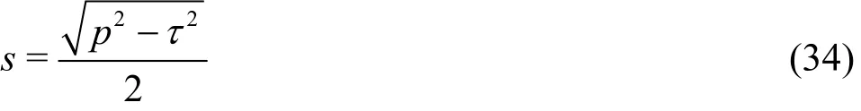
The partial dam break experiment is to test the accuracy of the current model. The experimental configuration is shown in Fig. 11. The reservoir is 1 m wide and 2 m long with a dry horizontal flood plain in the downstream of 3 m in length and 2 m in width.The dam is 2 m wide with a breach of 0.4 m located in the middle. The dam is represented as an elevation of the bed and the breach in the middle of the dam is created instantaneously at t=0 s, producing a flood wave across the dry flood plain. Three boundaries of the downstream flood plain are free outlet, while the boundaries of the reservoir are solid walls. The initial water depth in the reservoir is 0.6 m and the downstream flood plain is dry. A number of gauges are located at different locations to record the time series of the water depth. The locations of the gauges,as shown in Fig. 11, are listed in Table 2.
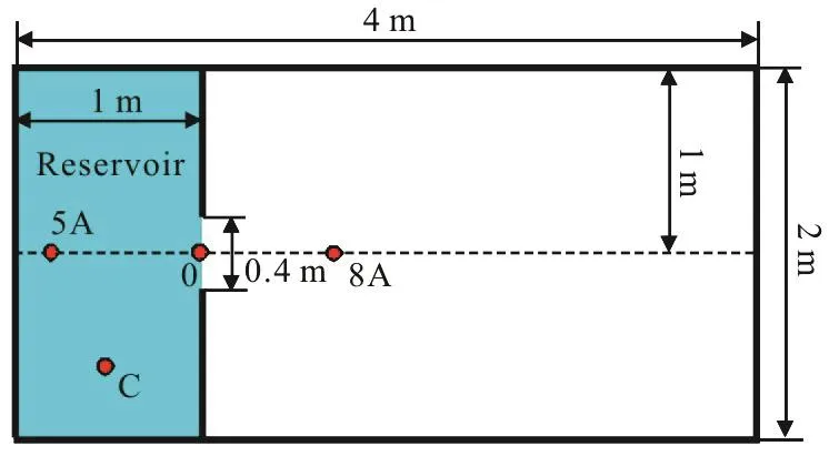
Fig. 11 (Color online) Sketch of partial dam break experiment and locations of gauge stations

Table 2 Locations of gauge stations
The computational domain is discretized by 400×200 cells with a uniform cell size of 0.01 m. The time series of the water depth at different gauges are compared in Fig. 12. After the dam break, a shock wave is formed and propagates toward the downstream direction of the floodplain. At the same time, a rarefaction wave appears in the reservoir, which drops the water surface in the reservoir. The computed water surface at the stations “5A” and “C” agree very well with the experimental observations. It can be observed that the water surface in the upstream reservoir oscillates significantly at the beginning due to the boundary reflection. The station “0” is located at the center of the breach and the depth hydrography descends to the minimum as soon as the dam fails.Then, the graph shows a rising of the water depth due to the lateral water propagation, as 2-D effects. The slight discrepancy may be due to the fact that the 2-D SWEs cannot exactly capture all three-dimensional features of the flow. At the station “8A”, the predicted water depth and the wave arrival time agree perfectly with the observation data. Therefore, it can be concluded that the overall accuracy of the current model for simulating the partial dam break flow is satisfactory.
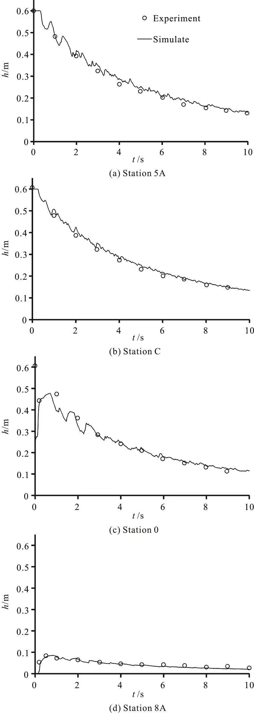
Fig. 12 Results of partial dam break experiment
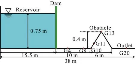
Fig. 13 (Color online) Sketch of the experimental setup and locations of gauges
2.5 Laboratory dam-break over a triangle obstacle
The presented numerical model is applied to a laboratory test of a dam-break inundation over a triangle obstacle, as is recommendated by the European research community, the concerted action on dambreak modeling (CADAM) project. The experiment was conducted in a 38 m long channel with the dam located 15.5 m away from the upstream end as shown in Fig. 13. A reservoir is in the upstream with a still water surface of 0.75 m and the downstream floodplain is dry initially. A symmetric triangle obstacle of 0.4 m in height and 6.0 m in length is installed in the downstream 13 m away from the dam. A constant Manning coefficient n=0.0125 is used throughout the whole domain, as is adopted by Liang and Marche[8]. The time series of the water depth are recorded at six gauges, located in the downstream 4 m(G4), 8 m (G8), 10 m (G10), 11 m (G11), 13 m (G13)and 20 m (G20) away from the dam as shown in Fig.13. The upstream end is solid wall and the down-stream end is free outlet.

Fig. 14 Time series of water depth at different gauges
The total simulation time is 90 s based on a grid with a uniform cell size of 0.05 m. Figure 14 shows the computed water depth at different gauges compared with the observation data. In the graphs, the simulated results of Liang and Marche[8]are also presented to demonstrate the accuracy of the present model. It can be found that the wave arrival time and the water depth are predicted accuratly at G4, G8, G10,G11 and G13. However, the water depth in the gauge G20 is overpredicted, which is also found in the simulation result obtained by Liang and Marche[8]. A possible explanation is that the flow between the tip of the obstacle and the outlet is very complex and the shallow water equations based on the hydrostatic situation are not suitable for this situation. It should also be noted that the wave arrival time at G20 is accurately predicted by the model, which is more important for the dam-break flood simulation.Overally, the comparison between the numerical results and the observation data is satisfactory at most gauge points and the wet/dry transitions are resolved accurately. This demonstrates that the present model is capable of simulatng the dam break flow over an uneven bed with a satisfactory accuracy.
2.6 Malpasset Dam break event
The Malpasset Dam is located on the Reyran River in southern France as shown in Fig. 15. It is a 66.5 m arch dam with the crest length of 223 m. The maximum reservoir capacity is 5.5×10⁷m3. The dam was collapsed in 1959 after an extremely heavy rain with a death toll of 421 people and considerable property damage in the downstream floodplain. A police survey was undertaken to get the maximum water levels along the Reyran River Valley after the dam break disaster and a physical model with 1/400 scale was set up in 1964 to measure the flood arrival time and the maximum water level at 9 points, located in the downstream floodplain. (see Fig. 15).

Fig. 15 (Color online) The elevation of topography with the locations of dam and experimental gauges (P)

Fig. 16 (Color online) The inundation map of water depth at t=30min

Fig. 17 Comparison of numerical results with experiment data at different gauges
Many researchers[23-24]used this case to test their numerical models, so do we in this study. In the computations, the computational domain is 550×220 grids with a uniform grid size of 30 m. The water level of the reservoir in the upstream is set to be 100 m and the downstream floodplain is assumed to be dry initially. The Manningʼs coefficient in the whole computational domain is set to n=0.033s/m1/3, the same as used by many researches[23-24]. Since there is no record about the actual breaching process of the dam,the dam is assumed to be removed instantaneously.Figure 16 shows the water depth and flood distributions at =30 min
t. The results of experimental measurements in terms of the water levels and the wave arrival time are compared with the simulation results in Fig. 17. It can be found that the numerical results agree well with the observation data at most gauge points. Some discrepancies at some points may be attributed to the three-dimensional features of the flow that cannot be exactly captured by a depth-averaged 2-D model. The simulated results of Wang et al.[23]are also presented in Fig. 17, which are similar to the results of the present model. However, slightly better results of the present model can be observed in terms of the flood wave arrival time. Overally, it can be said that the present model can give a good prediction for the field scale applications.
3. Conclusions
An improved well-balanced 2-D shallow flow model is developed based on the finite volume method using the structured grid to simulate the shallow water flow over an irregular topography with wetting and drying fronts. In the model, the Godunov-type central upwind scheme is used to calculate the fluxes at the interfaces of cells. In comparison with the existing shallow water models[17,19]that also use the central upwind scheme, the improvements of the present model can be summarized as:
(1) The non-staggered grid system is used to define the bed elevation and the primary flow variables at the cell center. Thus, all cells in the computational domain are either fully wet or dry, which avoids the problem of handling partially wetted cells.
(2) The nonnegative reconstruction of the water depth method proposed by Liang[15]is implemented in the present model to track the stationary or wet/dry fronts. Since it is not required to adjust the wet/dry fronts in the no-staggered mesh, the established model can preserve the “lake at rest” steady state for the dry bed applications and resolve the wet/dry fronts accurately.
(3) The occurring of the negative water depth is a key factor that causes the instability of a model to simulate flows over an irregular terrain. The established model can guarantee the positivity of the water depth when the Courant number is less than 0.25. It is not required to redistribute the water depth and the velocity to deal with the negative water depth, which makes the model robust and stable in modeling the flow over an uneven terrain.
The developed model is tested using three benchmark tests, two experimental dam break flow experiments, and a real dam break flood to evaluate its performance. The good agreements between the numerical results, the analytical solutions and the measured data demonstrate that the model can preserve the C-property, capture the steady flows, and resolve the wet/dry fronts accurately and promise a wide application in the natural flood prediction and management.
猜你喜欢
新高考·高二数学(2022年3期)2022-04-29
Chinese Physics B(2022年3期)2022-03-12
陶瓷科学与艺术(2021年12期)2022-01-26
十几岁(2021年5期)2021-11-22
上海工艺美术(2021年4期)2021-04-24
金秋(2020年12期)2020-10-21
检察风云(2020年16期)2020-09-26
鸭绿江(2016年5期)2016-04-29
中国领导科学(2015年10期)2015-02-05

- 水动力学研究与进展 B辑的其它文章
- Call For Papers The 3rd International Symposium of Cavitation and Multiphase Flow(ISCM 2019)
- Investigation of the hydrodynamic performance of crablike robot swimming leg *
- Determination of epsilon for Omega vortex identification method *
- Transient curvilinear-coordinate based fully nonlinear model for wave propagation and interactions with curved boundaries *
- Tracer advection in a pair of adjacent side-wall cavities, and in a rectangular channel containing two groynes in series *
- Numerical simulation of transient turbulent cavitating flows with special emphasis on shock wave dynamics considering the water/vapor compressibility *