On the estimation for product of covariance matrices and its trace
2020-07-08 05:41-,,
四川大学学报(自然科学版) 2020年4期
-, ,
(1. School of Mathematics, Sichuan University, Chengdu 610064, China; 2. School of Computer and Data Engineering, Ningbo Tech University, Ningbo 315100, China)
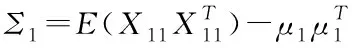
Abstract: In many statistical inference problems involving two populations respectively with covariance matrices Σ1 and Σ2, the product Σ1Σ2 and its trace tr(Σ1Σ2) need to be estimated. Firstly, we construct some equivalent estimators of Σ1Σ2 and unbiased estimators of and (Σ1Σ2)m for any positive integers m and n. Secondly, by using the equivalent estimators of Σ1Σ2, we show that some existing estimators of tr(Σ1Σ2) are equal. Finally, it is proved that two existing test statistics for testing the equality of two covariance matrices are asymptotically equivalent.
Keywords: Covariance matrix; Estimation; Statistical inference; Equivalence
1 Introduction
Consider twop-dimensional populations respectively with the mean vectorμiand covariance matrixΣi,i=1,2. The estimate of tr(Σ1Σ2) is essential and frequently encountered in multivariate statistical analysis, in particular, in two-sample covariance matrices testing problem. For example, one wants to test the hypotheses
H0:Σ1=Σ2vs.H1:Σ1≠Σ2
(1)
In the literature, the distance function between the null and alternative hypotheses is usually given by

(2)
where
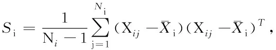
Note thatA1andB1are unbiased and location-invariant (i.e., not depending on the mean vectors) estimators ofΣ1Σ2and tr(Σ1Σ2), respectively, and the latter has been employed to construct the test statistic for the testing problem (1) in Ref. [3]. We also remark here that computingA1andB1requireN1p2+N2p2+p3andN1p2+N2p2+p2multiplications, respectively.


A straightforward calculation shows that
Σ1=E((X11-X12)(X11-X13)T)
and
Σ2=E((X21-X22)(X21-X23)T),
which leads to
Σ1Σ2=E((X11-X12)(X11-X13)T
(X21-X22)(X21-X23)T).
By covering all possible combinations, which is the essence of theU-statistics formulation, the second estimator ofΣ1Σ2is given as
(X1i-X1k)T(X2l-X2s)(X2l-X2t)T
(3)
(X2l-X2s)(X2l-X2t)T(X1i-X1j).
Note thatA2andB2are unbiased and location-invariant estimators ofΣ1Σ2and tr(Σ1Σ2),respectively. Obviously, computingA2andB2needN1(N1-1)(N1-2)p2+N2(N2-1)(N2-2)p2+p3andN1(N1-1)(N1-2)p2+N2(N2-1)(N2-2)p2+p2multiplications, respectively.
Noticing that
E((X11-X12)(X11-X12)T)=2Σ1
and
E((X21-X22)(X21-X22)T)=2Σ2,
we also have
(X21-X22)(X21-X22)T).
Hence, the third unbiased and location-invariant estimator ofΣ1Σ2is proposed as
(X1i-X1j)T(X2k-X2l)(X2k-X2l)T
(4)
Compatibly withA3given by (4), the third estimator of tr(Σ1Σ2) can be repressed as
(X2k-X2l)(X2k-X2l)T(X1i-X1j).
In Ref. [6], by virtue ofB3, the test statistics for testing multi-sample sphericity and identity of covariance matrices are constructed. Note that computingA3andB3takeN1(N1-1)p2+N2(N2-1)p2+p3andN1(N1-1)p2+N2(N2-1)p2+p2multiplications, respectively.
From
and
we have
Σ1Σ2=
(5)
By replacing four terms on the right hand side of (5) with their correspondingU-statistics respectively, the fourth unbiased and location-invariant estimator ofΣ1Σ2can be obtained as
(6)
Correspondingly, the compatible estimator of tr(Σ1Σ2) is given as
(7)

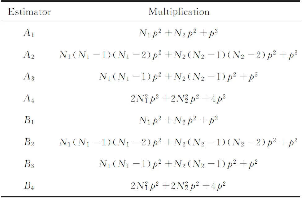
Tab.1 Computational complexity of the estimators
Theorem2.1A1=A2=A3=A4and thenB1=B2=B3=B4.
(8)
(N1-1)(N2-1)S1S2
(9)
-(N1-1)(N2-1)S1S2
(10)
-(N1-1)(N2-1)S1S2
(11)
(12)
Substituting (9),(10) into (8) yieldsA4=A1.
Some straightforward calculations indicate thatA2=A4andA3=A4, respectively. This completes the proof of this theorem.
Remark1We recall that the matrix estimatorsA2,A3andA4are constructed by the idea ofU-statistics. It particularly indicates that some desirable properties such as consistency ofAi,i=2, 3, 4,can be obtained conveniently based on the theory ofU-statistics which does not depend on the underlying distributions.
Remark2Note that the estimatorsB1,B3andB4have been directly utilized by Refs. [3], [6] and [5] respectively. However, to our best knowledge, there do not exist literatures presenting the relationship among these estimators. Theorem 2.1 asserts that these estimators, though having different forms and computational complexities, are exactly the same as tr(S1S2).
3 Unbiased estimators for more general case

For mutually different indicesi1,…,im,j1,…,jmand different indicesk1,…,kn,l1,…,ln, we have
(2 Σ1)m
and
(2Σ2)n.
Therefore,
(13)
(X2kb-X2lb)T)(X1i1-X1j1)
(14)
Similarly, we can obtain the unbiased and location-invariant estimators of (Σ1Σ2)m,tr((Σ1Σ2)m) and (tr(Σ1Σ2))mas follows.
4 Relationship between two existing test statistics
For the testing Problem (1), Ref.[5] constructed the following test statistic:
whereB4is given by (7) and
Later, for same testing problem, another test statistic was proposed in Ref. [3] as
whereni=Ni-1,B1is given by (2) and
withf=Ni(Ni-1)(Ni-2)(Ni-3) and

Under the assumption
(15)
Next, we show that the test statisticsTLCandTSare asymptotically equivalent.
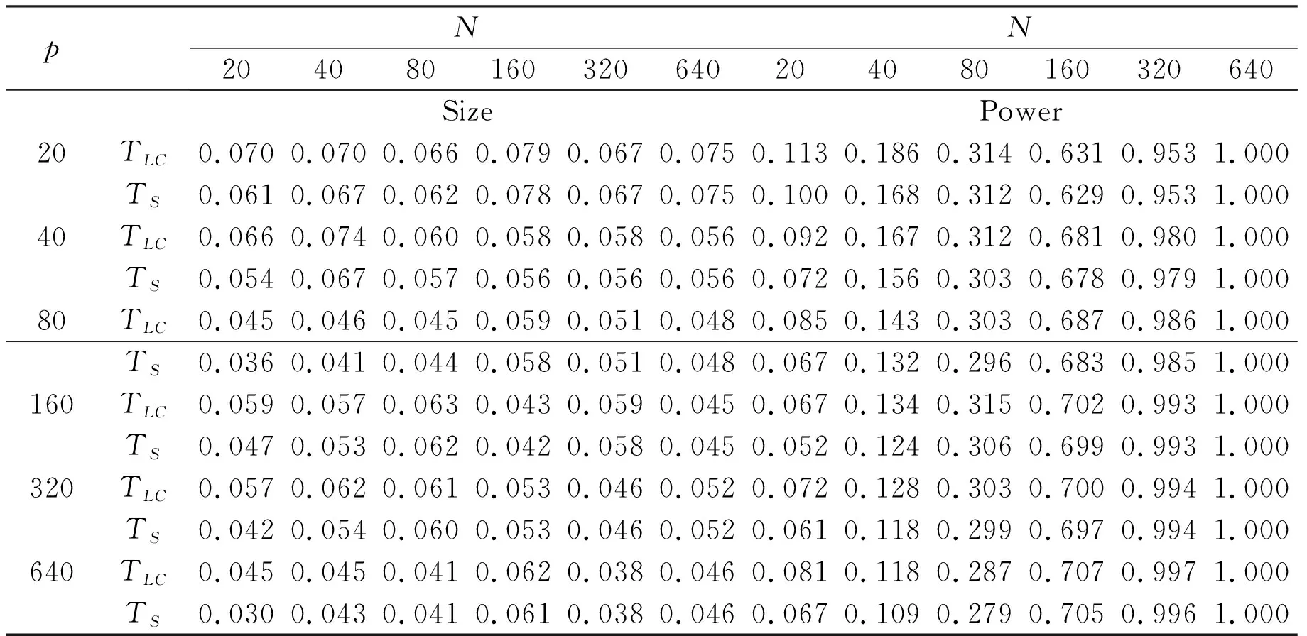
Theorem4.1TS It is easy to see thatβ<1 due toni=Ni-1,i=1, 2, which leads toTS Moreover,βcan be rewritten as which indicates thatβ→1 and thenTS-TLC→0 as min{N1,N2} tends to infinity. As a consequence, the fact thatTS-TLC→0 as min{N1,N2}→∞ in Theorem 4.1 also indicates that the test, proposed by Ref. [3] under the assumption (15), can be justified under the assumptions in Ref. [5], in which no relationship betweenpandNiis imposed. Tab.2 provides the empirical sizes and powers ofTLCandTSby 1000 Monte Carlo replications withN1=N2=Nand the nominal significance levelα=0.05. As showed in Table 2, whenNis small,TLCpossesses larger power thanTS, whileTShas smaller size thanTLC;the difference of sizes or powers betweenTLCandTSdecreases gradually asNincreases; particularly, whenN=640, the sizes or powers ofTLCandTSare almost the same. Therefore from the above statements, we may conclude thatTLCandTSare asymptotically equivalent. Tab.2 Empirical sizes and powers of TLC and TS
5 Conclusions