
Analysis of anomalous transport with temporal fractional transport equations in a bounded domain
2023-12-02 09:22KaibangWu吴凯邦JiayanLiu刘嘉言ShijieLiu刘仕洁FengWang王丰LaiWei魏来QibinLuan栾其斌andZhengXiongWang王正汹
Chinese Physics B 2023年11期
关键词:王正
Kaibang Wu(吴凯邦), Jiayan Liu(刘嘉言), Shijie Liu(刘仕洁), Feng Wang(王丰),Lai Wei(魏来), Qibin Luan(栾其斌), and Zheng-Xiong Wang(王正汹)
Key Laboratory of Materials Modification by Beams of Ministry of Education,School of Physics,Dalian University of Technology,Dalian 116024,China
Keywords: anomalous transport,temporal fractional transport equation,Caputo fractional derivatives,memory effects,hollow temperature profiles
1.Introduction
The mechanism of anomalous particle transport is one of the most significant issues in magnetically confined plasmas.In ordinary transport theory,the Brownian random walk model states that interactions between particles occur via collisions,which can be modeled by the Langevin equation.With the assumption that random forces are independent of the particle displacementsr, the solution to the Langevin equation gives〈r2〉∼t, meaning that the mean square displacement is linearly dependent on timet.However, in recent years, anomalous transport with a scaling law〈r2〉∼tβ(β/=1) has been observed in many experiments and simulations.[1–7]The value ofβcan represent different processes: 0<β< 1 for subdiffusion,β= 1 for ordinary diffusion, and 1<β< 2 for super-diffusion.Sub- and super-diffusions refer to particles diffusing more slowly and more quickly than in ordinary diffusion.
In magnetically confined plasmas,the Brownian random walk model based on collisions fails to explain experimental results due to collective behavior arising from the Coulomb force.In ordinary transport theory, the scaling law isD∝1/B2,[8]whereDis the diffusion coefficient andBis the magnitude of the magnetic field.However, Bohm experimentally determined the scaling law of diffusion to beD∝1/B,[9]which can be theoretically derived using the two-dimensional guiding center model.[10,11]In this model, due to theE×Bdrift motion of the guiding center,the velocity correlation can be transformed into an electric field correlation,which implies that the Coulomb force influences the diffusion process.
In Refs.[12–15], the decorrelation trajectory (DCT)method was proposed as a method to calculate diffusion coefficients.In this method, a global ensemble is divided into many sub-ensembles.In each sub-ensemble, the fluctuating electrostatic potentialφ(x,t) has a fixed value at the starting point, i.e., atx= 0 and att= 0, and therefore the velocity of the guiding center of each sub-ensemble is expressed as ∇φ(0,0)×ezas a result ofE×Bdrift.Furthermore, in each sub-ensemble, the decorrelation trajectory can be determined from the Hamiltonian equations of motion,along which the Eulerian correlation is calculated.Assuming that the Lagrangian velocity correlation in the sub-ensemble is equal to the Eulerian correlation, the diffusion coefficients can be calculated from the Lagrangian velocity correlation and related to the Kubo number defined asK ≡Vτc/λc,whereV,τc,andλcare the typical velocity of the particles, the correlation time,and the correlation length, respectively.Utilizing the DCT method yieldsD∝K2forK ≪1,andD∝Kγ,γ<1 forK ≫1.When the guiding center is undergoingE×Bdrift motion,the Kubo number can be written asK=ετc/(Bλ2c), whereεis the amplitude of electrostatic potential fluctuations.Therefore,K ≫1 implies that the system has strong turbulence due to the large amplitude of potential fluctuations.As particles encounter strong potential fluctuations,they are trapped by the fluctuations and undergo periodic motion.[12,16]As a result,it is possible that they diffuse more slowly than in the ordinary model and the system is in a sub-diffusive process.
In Refs.[12,17],the hybrid kinetic equations are utilized to obtain the evolution of the density profile,
whereL(τ)is the Lagrangian velocity correlation.For an ordinary transport process, the amplitude of the fluctuation is small, implyingK ≪1.Utilizing the DCT method yieldsL(τ)≈(ε/Bλc)2e-τ/τcsuch that the velocity correlation has an exponential decay and becomes insignificant asτ>τc.Sinceτccan be thought of as a short time scale,n(x,t-τ)≈n(x,t) can be assumed ift ≫τc, meaning that the density profile at timetdoes not relate to its past history.However,for an anomalous transport process, strong turbulence with large amplitude of fluctuation (K ≫1) has significant effect on particle motions, then the DCT method givesL(t)∼t-γ(1<γ<2)stating that the velocity correlation has power law decay and the assumptionn(x,t-τ)≈n(x,t)is no longer applicable.Thus,the density profile at timetis influenced by its past history as illustrated on the right-hand side of Eq.(1),implying that memory effects do exist.Moreover, due toL(t)∼t-γ,manipulating the integration in Eq.(1)yields scaling law〈r2〉∼tα(α=2-γ).[12,17]Hence,the density evolution of an anomalous transport process can be modeled by the temporal fractional diffusion equation.
Mathematically, the fractional derivatives are expressed as specific forms of integro-differential operators[18–20]that generalize the definition of conventional differentiation.There are many different types of fractional derivatives, including Riemann–Liouville, Gr¨unwald–Letnikov, and Caputo derivatives.In our work, we utilize the Caputo fractional derivative[21]
where Γ(x) is the Gamma function.It can be proven that the above formula returns to an ordinary first-order derivative asα →1.The Caputo fractional derivative is useful for solving initial value problems because it preserves the form of the initial conditions.Theoretical methods for solving ordinary fractional differential equations with the Caputo fractional derivatives are summarized in Ref.[20].The development of a numerical method to calculate Caputo fractional derivatives is significant to the study of complex problems as well.The Gr¨unwald–Letnikov formula[19]and L1 formula[22]are the two main numerical formulae used to calculate Caputo fractional derivatives.If 0<α<1, the Gr¨unwald–Letnikov formula can be used to obtain the first-order accuracy[19]and the L1 formula can improve the accuracy of order 2-α.[23]In Ref.[24], the L1-2 formula was used to achieve an accuracy of order 3-αby means of quadratic interpolation.The algorithms of numerical solution to other types of temporal fractional derivatives are discussed in Ref.[25]to investigate the memory effects in fractional-order chaotic systems.
The temporal fractional transport model in cylindrical coordinates has been studied in recent years in other academic fields.[26–31]In Ref.[12], the solution to the evolution of a density profile in an infinite domain in cylindrical coordinates in the absence of a source was derived.However,in real tokamaks,plasma particles are confined in a bounded domain and the solution to the diffusion equation can be expanded in terms of a series of orthogonal functions.In our work, we assume that a plasma system encounters a non-Markovian process with strong turbulence in a bounded domain.As mentioned in Refs.[12,16],plasma particles in a system with strong turbulence will be trapped by electric fields generated by large fluctuations.As a result,plasma particles diffuse slowly than ordinary.This kind of anomalous transport can be modeled using temporal fractional transport equations.Therefore,the goal of this work is to investigate memory effects on transport through numerical and analytical methods in a bounded domain.This paper is organized as follows: Section 2 briefly reviews the derivation of the temporal fractional diffusion equations.Section 3 compares the numerical results of density profiles under various orders of temporal fractional derivatives without sources and with uniform sources.At the end of Section 3,the application to off-axis heating processes is discussed.Section 4 presents a theoretical analysis, and Section 5 contains the summary and conclusions.
2.Derivation of the temporal fractional transport equation
In an ordinary transport process, particle jumps occur at regular, well-defined time intervals.However, in real situations, the time interval between successive jumps varies.Therefore, the continuous time random walk (CTRW) model can be introduced to generalize the Brownian random walk model.[32]In this model, particles are allowed to have an arbitrary jump length and waiting time expressed by probability distribution functions(PDFs).Furthermore,the temporal fractional diffusion equation can be derived from the master equation of this model.[33]In this paper, we concisely review the derivation of the temporal fractional transport equation from the CTRW model and the detailed derivation processes are provided in Refs.[12,32,33].Suppose that a particle is at positionx′at timet′,then stays atx′during a waiting timet-t′,and then jumps to positionx.We definef(x-x′)as the PDF of the jumpx-x′andψ(t-t′) as the PDF of the waiting timet-t′,such that the PDF of the process can be expressed asξ(x-x′,x′;t-t′;t′)=f(x-x′)ψ(t-t′).We further denote ˜was the Laplace transform of functionwand ˆvas the Fourier transform of functionvthrough
In one-dimensional space with the fluid limit(k →0,s →0),we assume that the system has a characteristic timeτcand a characteristic lengthλcimplying〈t〉 =τcand〈x2〉 =λ2c.
Hence, we have ˜ψ(p)≈1-τcpand ˆf(k)≈1-λ2ck2.Substituting them into Eq.(4)gives
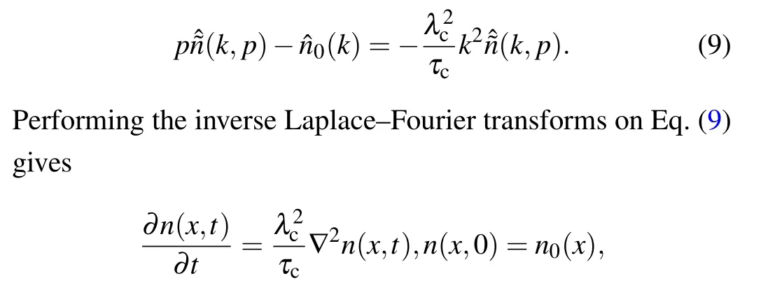
which returns to the ordinary diffusion equation.

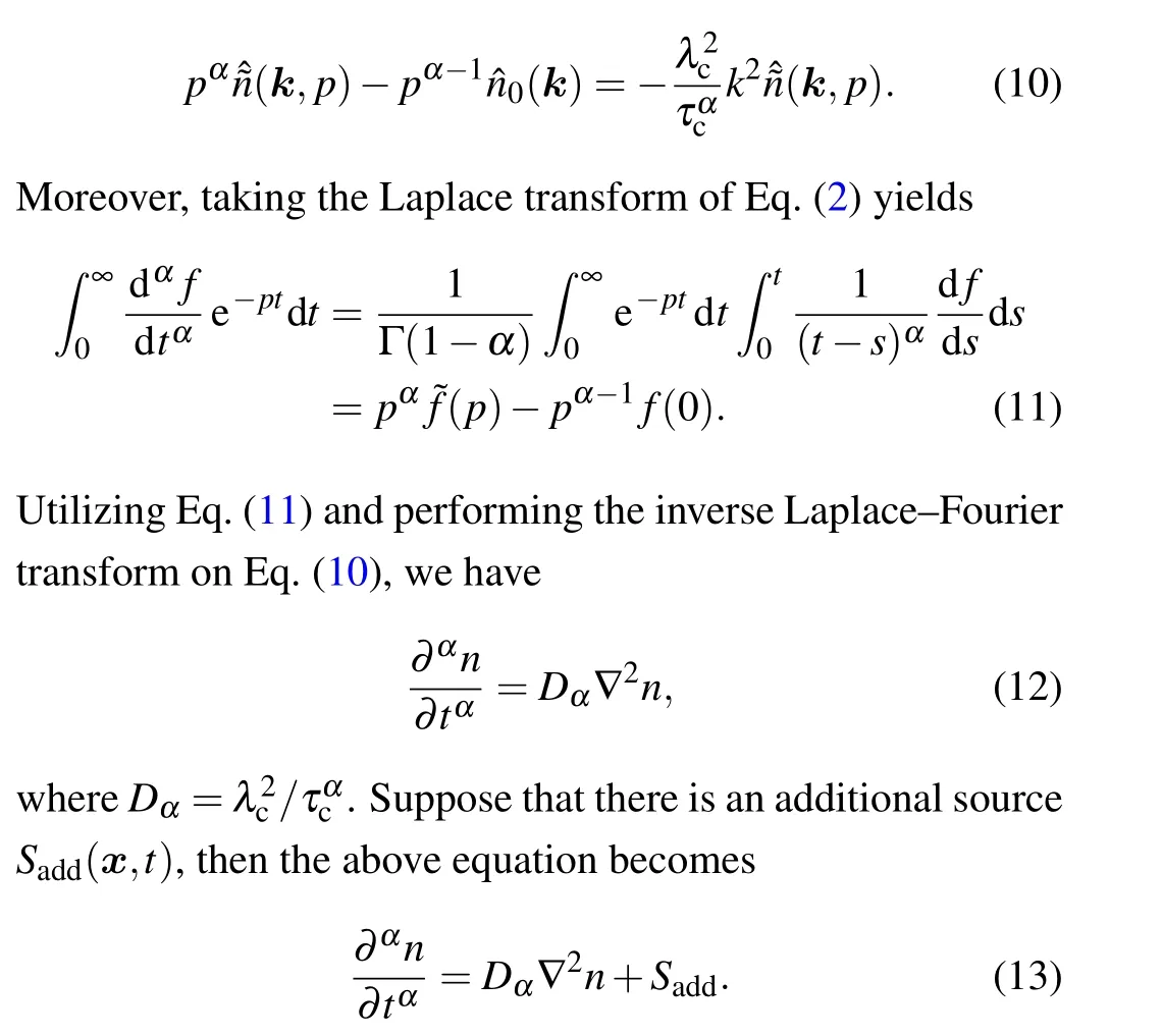
Ifα=1,the transport process is Markovian.If 0<α<1,the transport process is non-Markovian, and the memory effects have an influence on the transport process.In other words,αmeasures the influence level of the memory effects.
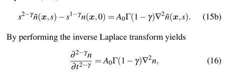
In Refs.[12,17],it was shown that the temporal fractional transport equation can be derived by the DCT method.Based on the DCT method,the asymptotic form of velocity correlation can be assumed to readL(t)≈A0t-γ(1<γ<2),whereA0is a constant and Eq.(1)becomes
Taking the Laplace transform on Eq.(14),we haveEquation(15a)can be rewritten as Eq.(16) is consistent with Eq.(12) ifα=2-γandDα=A0Γ(1-γ).Thus, the temporal fractional transport equation derived from the CTRW model is consistent with that derived from the DCT method.
3.Numerical results
In cylindrical coordinates,with a constant diffusion coefficient,the temporal fractional diffusion equation reads
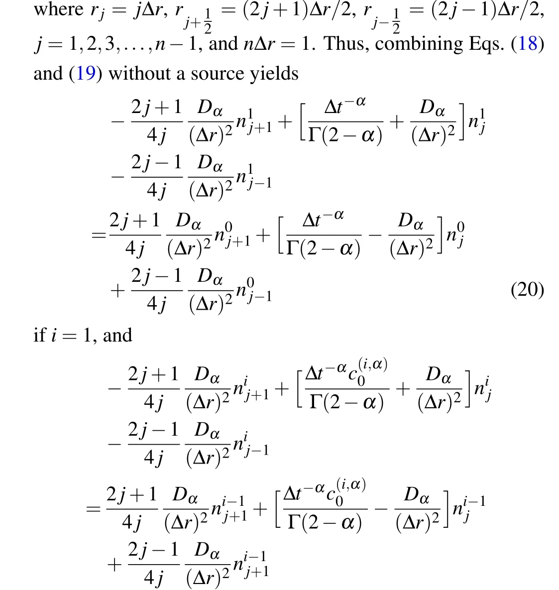
Note that the dimensionless variables are defined asr/a →r,t/t0→t,Dαtα0/a2→Dα, whereDαis the characteristic diffusion coefficient,ais the minor radius, andt0is the characteristic particle confinement time.Furthermore,the dimensionless variables of the source and the density are defined asSadd/S0→Saddandn/n0→n, wheren0is the characteristic diffusive scale of the density andS0=n0/tα0is the characteristic scale of the source.In Ref.[24],the authors developed the L1-2 formula,which expresses the temporal fractional partial derivative at timetiat positionrjas
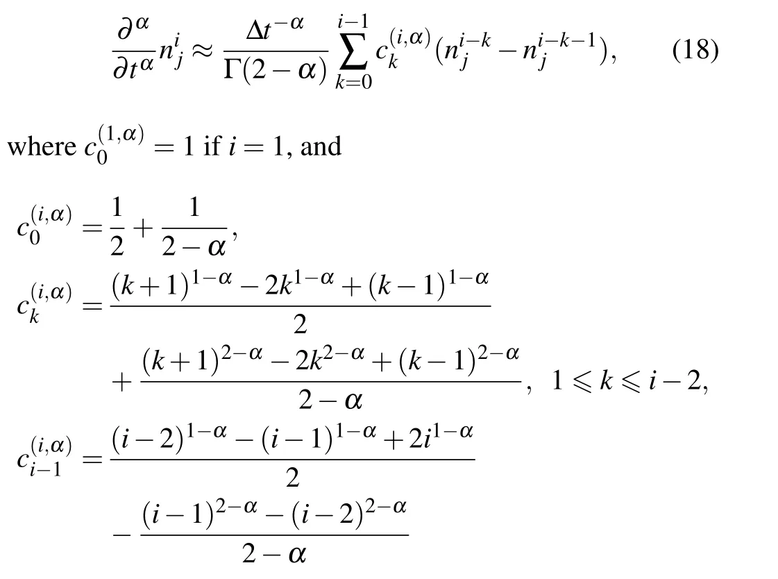
ifi≥2 and i∆t=ti.Since the authors utilized the explicit scheme for the temporal fractional partial differential equation, we apply the Crank–Nicholson method to improve the numerical stability in our work and the spatial partial derivative can be approximated as

so that we can investigate the effect ofαon the evolution of density profiles.Next,we numerically solve Eq.(13)with and without sources.
3.1.Without sources


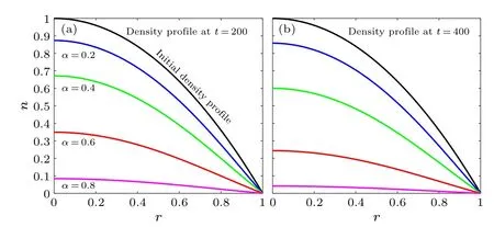
Fig.1.Density profiles at times t =200 and t =400 without sources.Comparing the blue, green, red, and magenta curves at t =200 and t =400, it is found that a smaller α leads to slower particle diffusion.Thus,the value of α controls the diffusion rate of the density.
3.2.With uniform sources
Next,we investigate the evolution of density profiles with sources.In this situation,the particles diffuse and also increase in number due to the injection from the sources.As a result,the diffusion and source terms eventually balance out,so that the system arrives at a steady state.Hence,in the steady state
we have
which implies that the form of the density profile at the steady statensis independent ofαand depends onSadd.We assume that the initial conditionn(r,0)=0 and that the source term is a constant,i.e.,Sadd=const.Therefore,the solution to Eq.(22)is
Thus,in the steady state,ns(r)=(1-r2)/4 and the total number of particles at steady stateNs=π/8 can be obtained ifDα=0.01 andSadd=0.01 are assumed.
Figure 2 illustrates that all of the curves approachns(r)=(1-r2)/4 at different speeds depending onα.For instance,Fig.2(d)reveals that the magnitude ofNtotforα=0.8 is larger than that forα=0.2,indicating that a largerαleads to a faster approach of the density profile towardns(r).Moreover,from the magnitude ofNtotfor eachαat each moment, it is found that the density profiles grow faster at the beginning and then slow down.Detailed data are listed in Table 1.
Thus,the simulation reveals that asα →1,the diffusion rate increases.As a result, the density decreases faster forα=0.8 than forα=0.2 without sources,and the density increases faster forα=0.8 than forα=0.2 with sources.
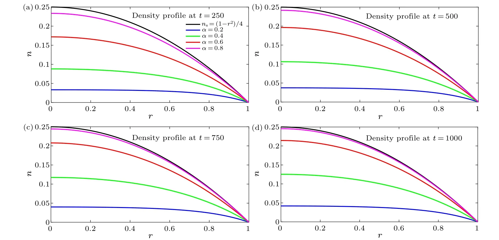
Fig.2.The evolution of the density profiles at different moments and different α with Sadd =0.01.The black curves represent the density profile ns(r)=(1-r2)/4 in the steady state and each curve approaches ns with a different speed depending on α.
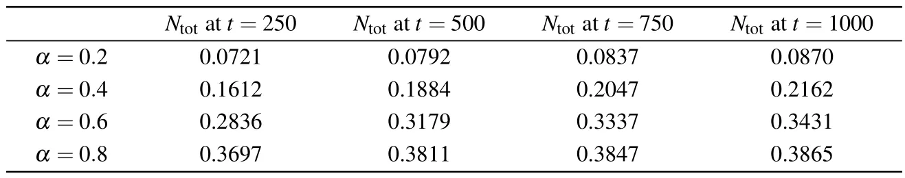
Table 1.The total number of particles Ntot at different moments.
3.3.Applications to magnetically confined plasmas
So far,as mentioned in Subsections 3.1 and 3.2,it is found that as the temporal fractional orderαdeceases,the rate of diffusion decreases as well.Therefore,αcan be thought of as the measure of the memory effects.In the derivation of the temporal fractional transport equation, we start with the CTRW model of particles.Supposing that these particles carry energy, as they jump from positionx′to positionxduring a waiting timet-t′,energy transport may occur.Therefore,we may utilize the CTRW model to simulate the evolution of the temperature profile and Eq.(8)can be rewritten as
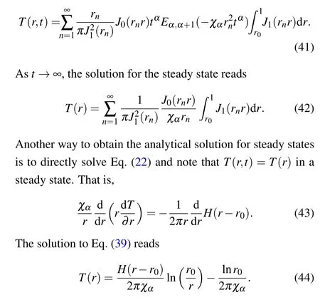
whereTis the temperature,χαis the thermal conductivity,andHaddis the heating source.Hence, the memory effects on the anomalous transport of temperature can be investigated through Eq.(24).In early works, hollow temperature profiles were observed in steady states under off-axis heating,[34]and theories based on nonlocal transport by utilizing the spatial fractional transport equation in Markovian processes were developed.[35–38]In order to investigate memory effects on the formation of hollow temperature profiles under off-axis heating processes,we assume the heating source to be of the formHadd=Hee-(r-r0)2/a2,wherer0=0.75,a=0.05,andHeis a constant,such that
The initial and boundary conditions are the same as those in the above section.Figure 3 shows the evolution of temperature profiles for variousα.In this work, the temperature profiles in the steady stateTs(r) can be obtained by solvingχα∇2T+Hadd=0 using the finite difference method.
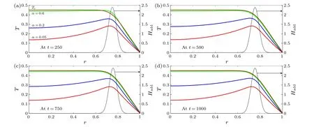
Fig.3.When a plasma system is heated at its edge,a hollow temperature profile can result.In a steady state,the temperature profile Ts can be obtained using the finite difference scheme.However,for a system with α approaching zero,the memory effects weaken the heat conduction,such that the hollow temperature profile can be sustained for a longer time.
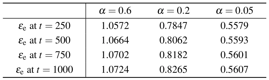
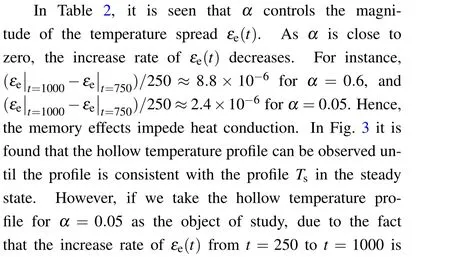
Table 2.The temperature spread εe(t) for different α at different moments.
When a plasma system undergoes an off-axis heating process, heat is first conducted from the location of the heating source.As shown in Fig.3, heat in a system withα=0.6 is conducted faster than that withα=0.2 andα=0.05, such that the temperature profile from the core tor0= 0.75 forα=0.6 is flatter than that forα=0.2 andα=0.05.Moreover,it is found that temperature profiles have local minima at the core for eachαand that the maxima are close to the position of the heating source.Hence,hollow temperature profiles are formed.In order to investigate memory effects on hollow temperature profiles,we further define the temperature spreadεe(t)as
and the simulation results are listed in Table 2.

4.Theoretical analysis


The solution to the above equation can be derived through the Laplace transform.Therefore,we have
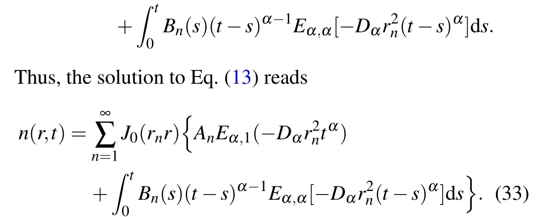
The first term in the braces on the right-hand side of Eq.(33)is the solution in the absence of an additional source term,while the second term represents the effect of the additional source term on the solution.Moreover, Eq.(33) reveals that the solution can be expanded in a series of Bessel functions,unlike the solution for an unbounded domain derived in Ref.[12].Ifα →1,Eq.(13)returns to an ordinary diffusion equation and Eq.(33)becomes
which is consistent with the solution to the ordinary diffusion equation.

Fig.4.The decay of the function Eα,1(-tα) with time for different α.The slopes of all curves are steep in the beginning and then become shallower.This is consistent with the simulation results,showing that the total number of particles decreases rapidly at the beginning and more slowly at later times.
We next study the situation without an additional source,so the second term on the right-hand side of Eq.(33) can be ignored.Then the solution reads
To investigate the effect ofαon the evolution of the density profile, we may setDαr2n= 1 for simplicity.Figure 4 shows that as time increases,Eα,1(-tα) decreases and eventually approaches zero.Moreover, it is found that the rate of decay depends onα.For instance,att=7,forα=0.99999,Eα,1(-tα)≈0,while forα=0.2,Eα,1(-tα)≈0.375.Hence,asαincreases,the decay rate of the density increases as well.
The asymptotic behavior of the Mittag–Leffler function is
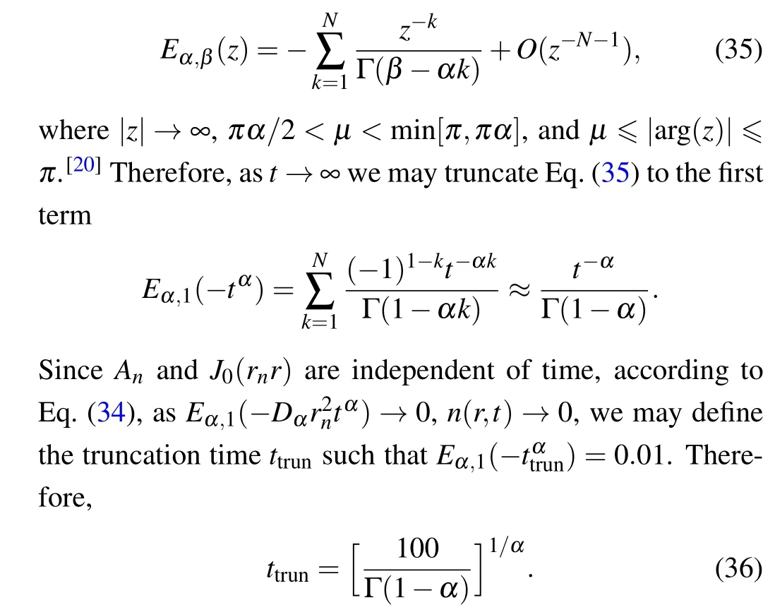
From Eq.(36), whenαapproaches zero, the truncation time approaches infinity.Whenα →1,the truncation time goes to zero.Thus,the smaller theαis,the longer the system spends for achieving a rare density state.
When a source is taken into consideration,the solution to Eq.(13)can be expressed as in Eq.(33).Ifα →1,corresponding to the ordinary diffusion equation,the factor(t-s)α-1in the integrand equals unity, so that this factor does not affect the density profiles.However, since 0<α<1, this factor cannot be disregarded.Moreover, the factorBn(t)(t-s)α-1arising from the source term implies that the density profile at positionrand timetis influenced by the past history of the source term through the factor(t-s)α-1.In other words,the factor(t-s)α-1strengthens the memory effects of the source term.Taking our work as an example, the initial conditionsn(r,0)=0 andSadd=constare assumed,soAn=0 andBnis independent of time.Therefore,combining Eqs.(28),(32),and(33),we obtain

We further assumeDαr2n=1 so as to study the influence ofαon the density profiles,and the above equation becomes
If we make Eq.(38) a function independent of time, i.e., in a steady state, the second term on the right-hand side should be much less than the first term, such that the second term can be ignored.Figure 2(d) shows that the density profile forα=0.2 has a larger difference fromns(r)=(1-r2)/4 than that forα=0.8, which implies that the value ofαdetermines how long a system needs to reach a steady state.To estimate the truncation time in order to ignore the second term on the right-hand side of Eq.(38), we may assume that the second term is 1% of the first term to obtain another truncation timettrun,s= [100/Γ(1-α)]1/α(s in the subscript denotes a steady state).Note that the form of this truncation time is the same as in Eq.(36),but the physical meanings are different.The ratio ofttrun,sforα=0.2 to that forα=0.8which means that the truncation timettrun,sforα= 0.2 is much greater than that forα=0.8.Thus, asαdecreases, the time required to reach a steady state increases.
To investigate the evolution of temperature profiles under off-axis heating processes,we assume that the heating source has the formHadd=Hee-(r-r0)2/a2,wherer0=0.75,a=0.05,andHeis a constant,such that
Substituting Eq.(39)into Eq.(24)and applying the initial conditionT(r,0)=0 yield
After a plasma system is heated from the edge,the heat starts to be conducted by Fick’s law.Therefore, a hollow temperature profile is formed.As time passes, the temperature at the core increases and the hollow profile flattens.When the plasma system is in a steady state, the temperature profile does not evolve with time,consistent with the brown curves in Fig.5.However,the time required to reach the steady state increases asαdecreases.Hence,the smaller theαis,the longer the hollow temperature profile can exist.This can also be concluded from the formulattrun,s=[100/Γ(1-α)]1/α →∞forα →0, implying that asαapproaches zero, the system requires an infinite amount of time to reach the steady state and the hollow temperature profile can be observed indefinitely.
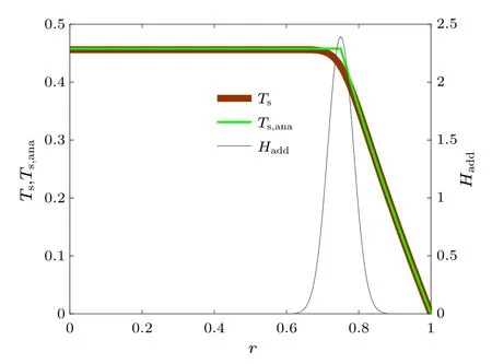
Fig.5.The temperature profile in a steady state can be numerically calculated through the finite difference scheme as shown by the brown curve denoted as Ts.It can also be analytically derived from Eq.(43),as shown by the green curve denoted as Ts,ana.The source profile for the numerical calculation has the form Hadd=Hee-(r-r0)2/a2 instead of the Dirac delta function.
5.Summary and conclusion
In this work,we have investigated the effect of a temporal fractional derivative on transport in a Fickian process with and without sources.The fractional order of the temporal derivative in Eq.(13)can be derived from the CTRW model and the DCT method.Moreover,Eq.(2)states that the time evolution of the density is affected by its past history,which means that the memory effects have a significant influence on anomalous transport.Whenα →1,memory effects abate and disappear,reducing the fractional diffusion equation to the ordinary diffusion equation.
When a source term is taken into account, the memory effects have an influence on the time needed to reach a steady state.As shown in Figs.2 and 3, asαincreases, the time required to achieve a steady state decreases.Hence,for a system in a sub-diffusive process with a source, the memory effects will prevent the system from reaching a steady state.Therefore, memory effects could be significant in allowing hollow temperature profiles to exist for a long time under off-axis heating.
It should be pointed out that non-local effects are also important to transport in Markovian processes, as investigated in Refs.[35–38].It would be interesting to consider both non-local and memory effects at the same time.In addition, the fractional orderαdepends on the Kubo numberK=ετc/(Bλ2c), which means that it depends on the magnetic fields and electrostatic fluctuations.In a real tokamak device,the magnetic field has spatial and temporal dependences,which implies thatαis a function of space and time.Moreover, asK ≫1 implying weak magnetic field or large electrostatic fluctuations in a system,the memory effects become significant to impede transport processes.Hence, our future work will focus on anomalous transport with spatial-temporal variance of the fractional orderα.
Acknowledgments
This work was supported by the National Key R&D Program of China (Grant No.2022YFE03090000), the National Natural Science Foundation of China (Grant No.11925501),and the Fundamental Research Fund for the Central Universities(Grant No.DUT22ZD215).
猜你喜欢
Chinese Physics B(2023年10期)2023-11-02
Chinese Physics B(2023年7期)2023-09-05
Chinese Physics B(2022年11期)2022-11-21
Chinese Physics B(2022年6期)2022-06-29
Plasma Science and Technology(2022年5期)2022-06-01
Plasma Science and Technology(2022年4期)2022-05-05
Plasma Science and Technology(2022年3期)2022-04-15
Plasma Science and Technology(2022年2期)2022-03-10
Plasma Science and Technology(2021年11期)2021-11-30
文艺生活(艺术中国)(2020年1期)2020-12-10

- Chinese Physics B的其它文章
- Optimal zero-crossing group selection method of the absolute gravimeter based on improved auto-regressive moving average model
- Deterministic remote preparation of multi-qubit equatorial states through dissipative channels
- Direct measurement of nonlocal quantum states without approximation
- Fast and perfect state transfer in superconducting circuit with tunable coupler
- A discrete Boltzmann model with symmetric velocity discretization for compressible flow
- Dynamic modelling and chaos control for a thin plate oscillator using Bubnov–Galerkin integral method