
Band structures of strained kagome lattices
2024-02-29 09:17LutingXu徐露婷andFanYang杨帆
Chinese Physics B 2024年2期
关键词:杨帆
Luting Xu(徐露婷) and Fan Yang(杨帆),†
1Center for Joint Quantum Studies and Department of Physics,School of Science,Tianjin University,Tianjin 300354,China
2Tianjin Key Laboratory of Low Dimensional Materials Physics and Preparing Technology,Department of Physics,Tianjin University,Tianjin 300354,China
Keywords: kagome lattice,strain,band structure engineering
1.Introduction
A kagome lattice is a special two-dimentional (2D)hexagonal Bravais lattice consisting of corner-sharing triangles.It has been discovered as a fertile land for realizing various exotic physics since introduced by Syˆozi in 1951.[1]Due to their frustrated lattice geometry and nontrivial band features,kagome lattices are predicted to be a promising platform for investigating novel physics such as frustration-driven magnetism,[2,3]quantum-spin-liquid states,[4–10]topological phases,[11–13]and electron correlations.[14]
Unfortunately, materials with kagome lattices are rare in nature.As an alternative approach to explore the physics related to kagome lattices, various artificial kagome systems,such as optical kagome lattices[15–17]and monatomic kagome layer grown on metal surfaces,[18]have been experimentally developed.The advantage of artificial kagome systems is that they allow the individual tuning of all system parameters in a wide range,and thus enable us to search for the predicted nontrivial features of kagome lattices in a much larger parameter space.For example, in natural kagome materials, parameters such as hopping energy, defect density and mechanical strain are difficult to control experimentally,but they can all be conveniently tuned in artificial kagome systems by simply varying the designs and geometries of the artificial lattices.
Mechanical strain has proven to be an important tool for engineering electronic band structures.[19–21]Over the past decades,extensive research has been carried out on the strain effect in graphene,[22–25]carbon nanotube,[26–28]MoS2,[29–31]WSe2,[32,33]and many other materials.In contrast,studies of strained kagome systems have just started;[34–38]a systematic investigation of the band structures of strained kagome lattice is still lacking.
In this work, we theoretically study the electronic band structures of a strained kagome lattice using both a tightbinding model and an antidot model based on a periodic muffin-tin potential.The main findings include: (i)The Dirac points of kagome lattice are shifted away from the corners of Brillouin zoom under applied uniaxial strain.In contrast to the situation in strained graphene,[23]the Dirac cones of strained kagome lattices never merge within the framework of the nearest-neighbor tight-binding model.However, in a more realistic model based on a periodic muffin-tin potential,the Dirac cones do merge with increasing compressive strain,causing band-gap openings at the Dirac points.(ii) When a stretching strain is applied inydirection, the flat band of the unstrained kagome lattice becomes highly anisotropic, forming a partially flat band with an area that is dispersionless alongkydirection whereas dispersive alongkxdirection.
The paper is organized as follows.In Section 2, we calculate the energy bands of the strained kagome lattice using the nearest-neighbor tight-binding model.In Section 3, we first introduce an antidot model for artificial kagome lattice,and then numerically investigate its band structures under uniaxial strain.The results and conclusions are summarized in Section 4.
2.Tight-binding approach to the strained kagome lattice
In this section, we investigate the band structures of the strained kagome lattice using the tight-binding approximation.Since the band structures of the kagome lattice are primarily characterized by coexistence of Dirac cones and a flat band,here we mainly focus on the shift of the Dirac cones and the reshaping of the flat band in response to applied uniaxial strain.
2.1.The tight-binding model for the kagome lattice
Figure 1(a) presents an illustration of the nearestneighbor tight-binding model for the strained kagome lattice.The kagome lattice is a triangular Bravais lattice with a unit cell composed of three inequivalent sites, which are labeled asA,B, andC, respectively.The three sites in the unit cell form a regular triangle, as indicated by the shaded region in Fig.1(a).The repeated Brillouin zone of kagome lattice is shown in Fig.1(b), where the first Brillouin zone is a regular hexagon with two independent cornersKandK′.
The tight-binding Hamiltonian of the kagome lattice reads[11,34]
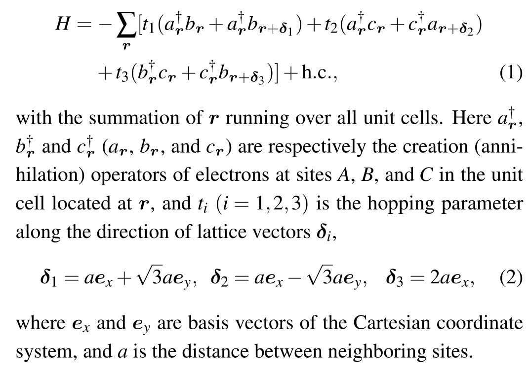
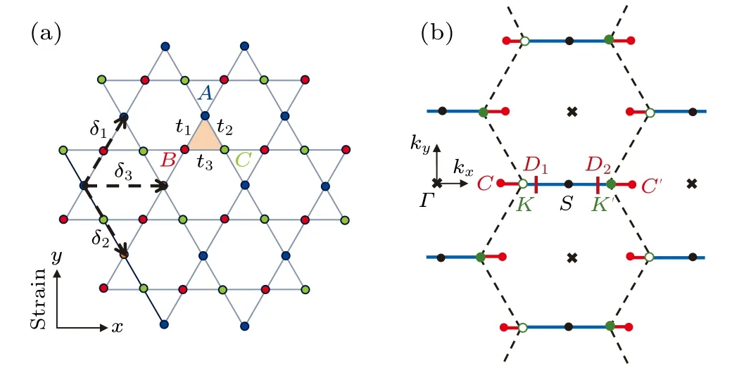
Fig.1.(a) The tight-binding model of the kagome lattice with only nearest-neighbor hopping terms.The three inequivalent sites in the unit cell are labeled as A, B, and C, respectively;ti (i=1,2,3)denotes the hopping parameter between the nearest neighboring atoms along direction δi.A uniaxial strain in y direction is modeled by a group of anisotropic hopping parameters t1=t2=t′and t3=t.(b)The repeated Brillouin zone of the kagome lattice.The central point Γ and two independent corners K and K′ are denoted by the black crosses, hollow green circles and solid green circles, respectively.When the lattice is strained in y direction,the Dirac points D1 and D2 are shifted away from K and K′ and located somewhere between C and C′.
By applying the Wannier transformation

Hereki ≡k·δi(i=1,2,3),satisfyingk1+k2=k3.
In an unstrained kagome lattice, the six-fold rotational symmetry ensurest1=t2=t3.However,as shown in Fig.1(a),an uniaxial strain applied inydirection breaks the rotational symmetry and consequently leads tot1=t2̸=t3.Assuming thatt1=t2=t′andt3=t, the anisotropy ratioαcan be defined asα ≡t′/t.The parameterαcharacterizes both the type and strength of the uniaxial strain, as explained as follows: (i) A decrease in inter-site distance always causes an increment of hopping parameter, and vise versa, and henceα>1(α<1)corresponds to the situation where a compressive strain(stretching strain)is applied alongydirection.(ii)Apparently,the further theαdeviates from 1,the stronger the applied strain is.
Meanwhile, as a reasonable approximation for weak strain,[23]we neglect the site shift in the strained lattice and assume that the lattice will keep its shape whenα ̸=1.Based on this assumption,a uniaxial strain applied inydirection can be modeled using a single parameterα,which greatly reduces the mathematical complexity.The eigenvalue equation ofℋkis consequently reduced to
2.2.Results and discussion
2.2.1.General features of energy bands

2.2.2.Shift of Dirac points
The shift of Dirac points are more visible in the energy bands plotted along thekxaxis.As shown in Fig.2(d),the intersection points of the two lower bands,i.e.,the Dirac points,move with applied strain.The horizontal position of the two Dirac points are calculated analytically as
Obviously,Dirac pointsD1andD2are symmetric with respect to theSpoint atkx=π/a[see Fig.1(b)].Therefore,in the following we discuss only the position ofD1.
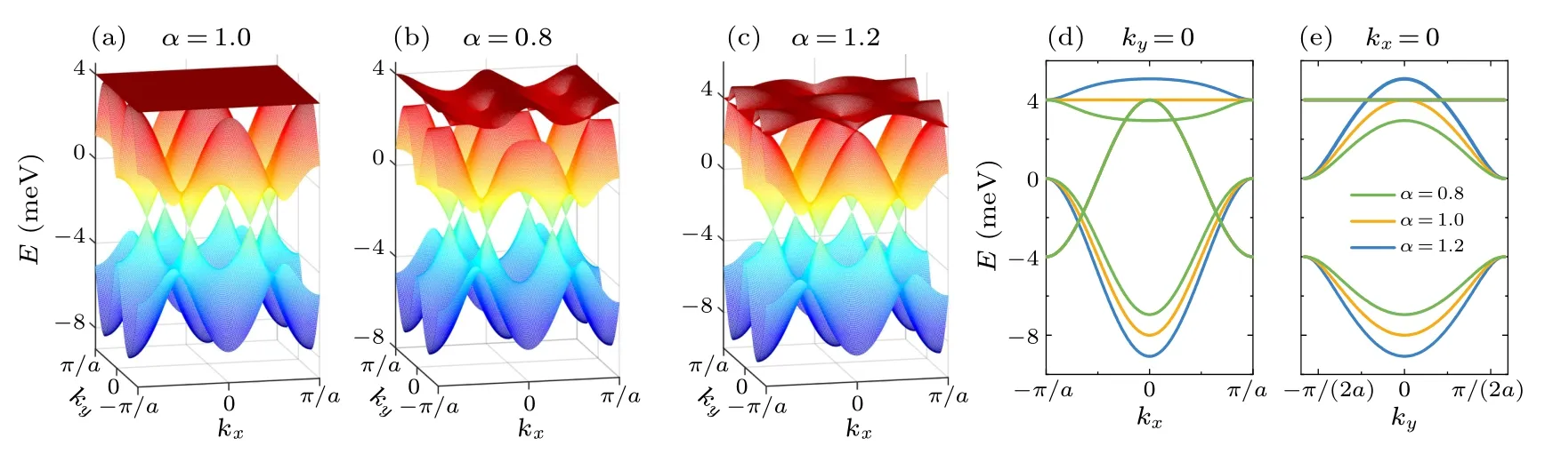
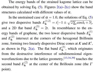
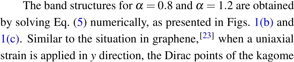
Fig.2.[(a)–(c)] Band structures of strained kagome lattices with various anisotropy ratio α ≡t′/t, calculated using a tight-binding model with only nearest-neighbor hopping.The lattice is (a) unstrained (α =1.0), (b) stretched (α =0.8), and (c) compressed(α =1.2)along y direction.[(d),(e)]Band structures plotted along(d)the kx axis and(e)the ky axis.The hopping parameter along x direction is set to t=t3=2 meV.
The movement of Dirac points in response to strain are summarized as follows.(i)For the kagome lattice stretched inydirection (α<1), the Dirac pointD1moves along theKCline [red lines in Fig.1(b)] towards theCpoint atπ/2a, andD1→Cwhenα →0.(ii) For the unstrained kagome lattice(α=1),D1lies exactly at theKpoint of the Brillouin zone,withkD1x=2π/(3a).(iii)For a lattice subjected to a compressive strain inydirection(α>1),D1moves towards theSpoint along theKK′line[blue lines in Fig.1(b)],andD1→Swhenα →∞.
In a word, compared to graphene where the Dirac cones merge under applied strain,[23]the Dirac cones of kagome lattice remain intact at any strength of uniaxial strain within the framework of the nearest-neighbor tight-binding model, indicating a more robust phase of semimetal.
2.2.3.Reshaping of flat band

3.Artificial kagome lattice under uniaxial strain
In this section, we numerically investigate the strain effects in artificial kagome lattices using an antidot model.Compared with the tight-binding model with only nearestneighboring hopping terms, the antidot model based on a periodic potential is more realistic in the sense that it provides the design of antidot patterns required for experimentally fabricating artificial kagome materials from conventional twodimensional electron gases(2DEGs).[40–42]
3.1.Antidot model for kagome lattice
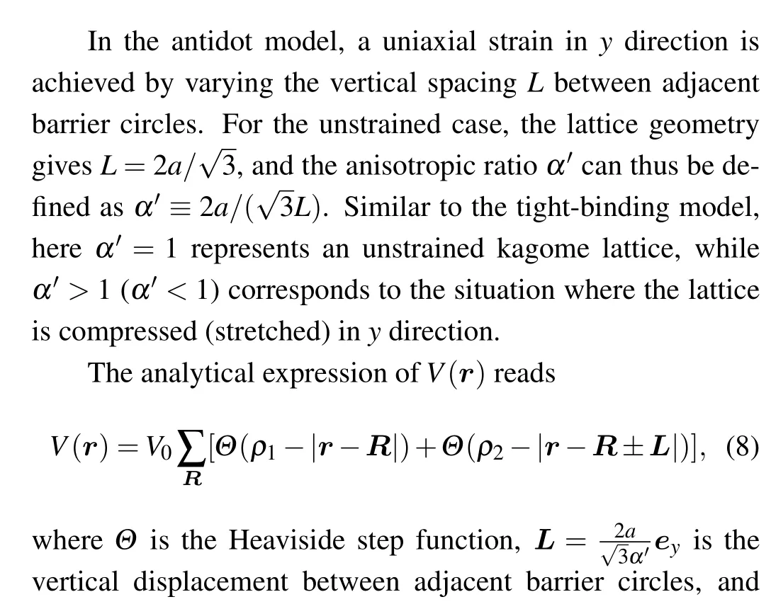
Two different antidot models have been proposed in the literature for realizing kagome lattices,[42,43]and here we adapt the design in Ref.[42].This model is based on a periodic muffin-tin potentialV(r)comprising two types of circular barrier regions whereV(r)takes a constant valueV0>0,as indicated by the blue circles in Fig.3(a).The radii of the large and small barrier circles are denoted byρ1andρ2, respectively, and the vertical spacing between nearest-neighboring circles is denoted byL.Most calculations in this section are performed withρ1/ρ2=3,because such a choice ensures that the large and small barrier circles in Fig.3(a) will touch the dashed lines simultaneously asρ1increases.Due to the repulsion from the barriers,the wave functions of electrons mainly distribute in the space between the barrier regions,forming an artificial kagome lattice with a horizontal inter-site distance ofa,as illustrated by the hollow circles in Fig.3(a).
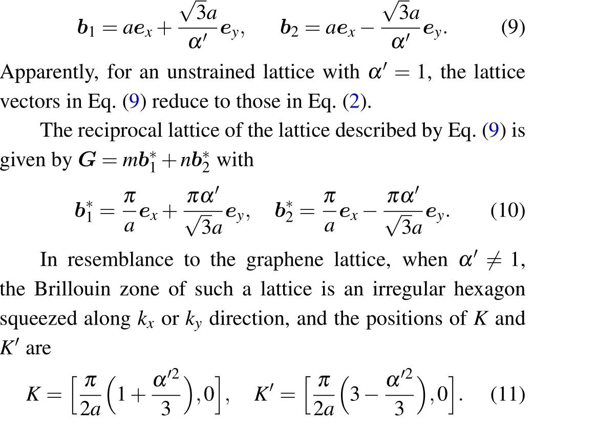
Fig.3.(a) Periodic muffin-tin potential for realizing the artificial kagome lattice.The potential function satisfies V(r)=V0 >0 inside the blue circles and V(r)=0 elsewhere.The large solid circles form a triangular lattice spanned by the lattice vectors b1 and b2, the angle between which changes with applied strain.Each large circle is surrounded by six small circles.The hollow circles located in the gaps between blue circles illustrate the sites of the kagome lattice.The lattice shown here is stretched along y direction with α′ =0.8.(b) The repeated Brillouin zone corresponds to the lattice shown in(a).The first Brillouin zone of the strained kagome lattice is a squashed hexagon.The Dirac points are located in the CC′ line when a uniaxial strain is applied in y direction.

3.2.Numerical method for band calculation
For an electron system subjected to the periodic potentialV(r)given by Eq.(8),the Bloch wave functionψk(r)satisfies the Schrödinger equation
3.3.Results and discussion
In the following we present the numerical results obtained using the antidot model described in Subsection 3.1.The calculation was performed witha= 25 nm andm*= 0.04me,wheremeis the free electron mass.These parameters are experimentally achievable by fabricating an antidot array onto a typical 2DEG using e-beam lithography.
3.3.1.Width of the flat band
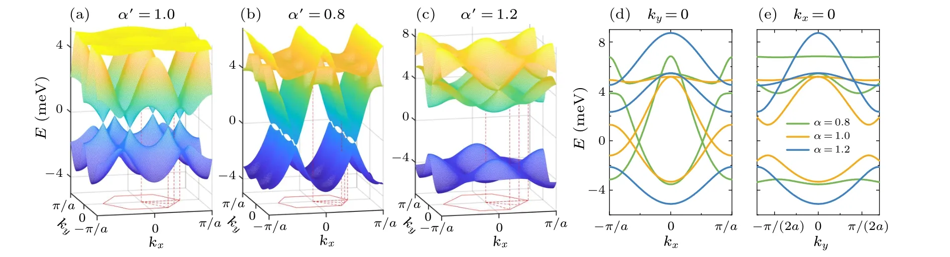
Fig.4.[(a)–(c)] The lowest three energy bands of strained kagome lattices with various values of α′, calculated using the periodic muffin-tin potential described in the main text.The lattice is(a)unstrained(α′ =1.0),(b)stretched(α′ =0.8),and(c)compressed(α′=1.2)along y direction.[(e),(f)]Band structures plotted along(e)the kx axis and(f)the ky axis.The bands are shifted vertically to move the Dirac points to zero energy.All calculations were performed with V0=200 meV,ρ1/ρ2=3,and β ≡ρ1/a=0.6.
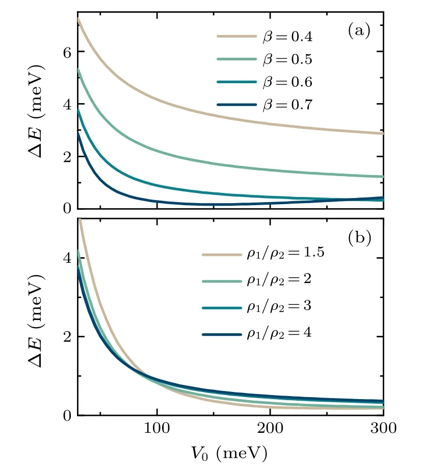
Fig.5.Band width ∆E of the flat bandversus barrier height V0 ofthe maffin-tin potential V(r)calculated(a)with ρ1/ρ2=3 and various values of β ≡ρ1/a,and(b)with various values of ρ1/ρ2 and β =0.6.
When eitherV0orβis small,the wave functions of electrons are not well localized to the regions of lattice sites illustrated by the hollow circles in Fig.3(a).In this situation,the antidot model cannot be well approximated by the tightbinding lattice model and therefore the obtained ∆Eofis large.As shown in Fig.5,∆Egenerally decreases with increasingV0andβexcept for the highV0region of the curve withβ=0.7.A small band width of ∆E=0.45 meV is obtained with parametersβ=0.6 andV0=200 meV;the calculations presented in Fig.4 were all carried out with this group of parameters.

3.3.2.Merging of Dirac points
To quantitatively present the movement of the Dirac points in response to applied strain,we introduce a parameterγto describe the relative position of the Dirac pointsD1andD2with respect to theSpoint[see Fig.3(b)].The parameterγis defined as
where|kC-kS|=|kC′-kS|=π/a.Obviously,γ=1 corresponds to the situation in which the Dirac pointsD1andD2are respectively shifted toCandC′,andγ=0 is reached whenD1andD2meet and merge at theSpoint.In addition, in the antidot model,it is noteworthy that bothKandK′move with applied strain due to the deformation of the lattice.Therefore,a parameterγKis similarly introduced to describe the relative position ofK,defined as
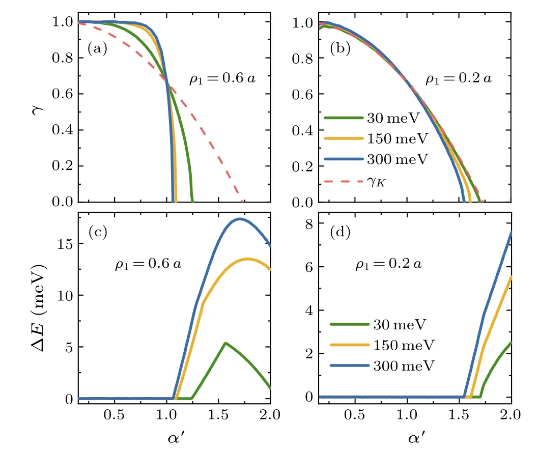
Fig.6.[(a), (b)] Relative position γ of Dirac points as a function of anisotropy ratio α′ for(a)β ≡ρ1/a=0.6 and(b)β =0.2,calculated with ρ1/ρ2 =3 and various values of V0.The dashed lines depict the position of the K point given by Eq.(17).[(c), (d)] Band gap ∆E at Dirac points as a function of α′, calculated with (c) β =0.6 and (d)β =0.2.
3.3.3.Partially flat regions in deformed flat bands
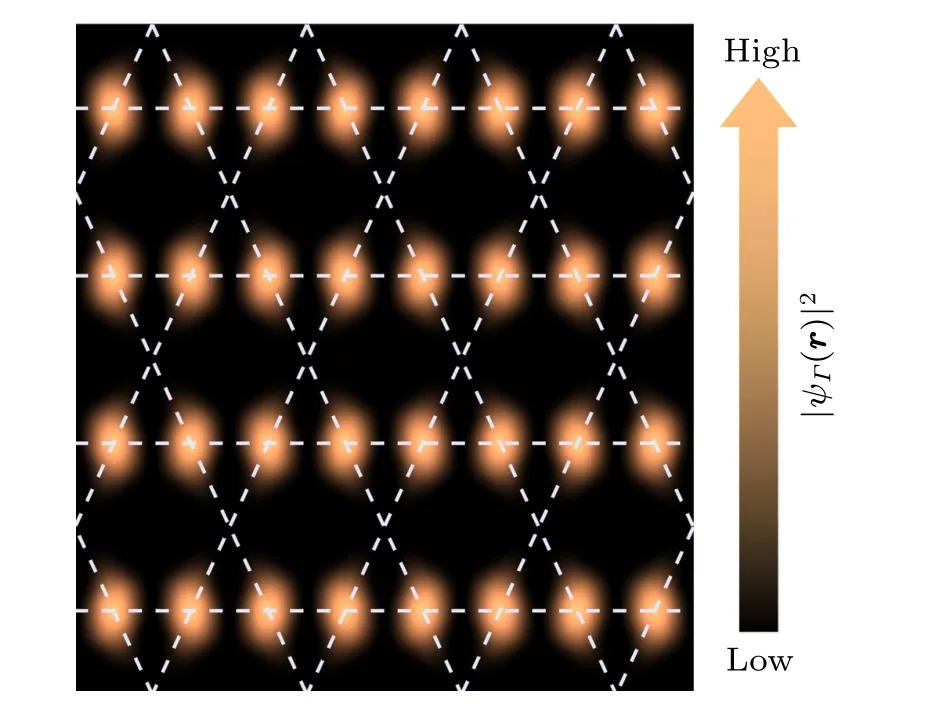
Fig.7.Probability density distribution of the Bloch state ψΓ(r)of band, calculated with α′ =0.8.Dashed lines illustrate the kagome lattice.The parameters of muffin-tin potential are the same as those in Fig.5.
4.Further discussion
4.1.Band structures along high-symmetry paths
To better illustrate the evolution of the band features in response to applied strain, we plot the band-structure data calculated using both the tight-binding model and the antidot model along the high-symmetry pathΓ–M–K–Γ–M′–K′.As shown in Fig.8, the band structures calculated using the tight-binding model always show characteristic van Hove singularities at both theMandM′points, irrespective of applied strain.However, for the band structures calculated using the antidot model,the van Hove singularity at theMpoint disappears whenα′=0.8 whereas that at theM′point disappears whenα′=1.2,as illustrated in Figs.9(b)and 9(c).
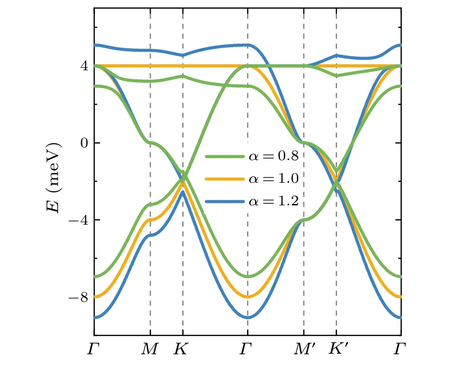
Fig.8.Plots of the band-structure data in Fig.2 along the highsymmetry path.The corresponding Brillouin zone is illustrated in the left panel of Fig.9(a).
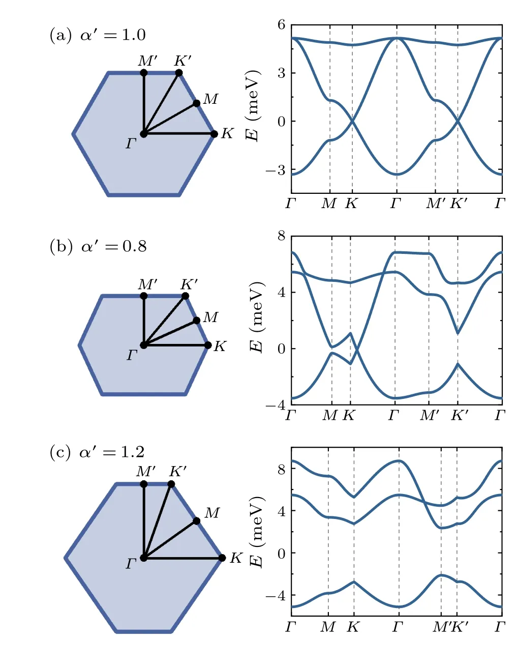
Fig.9.Plots of the band-structure data in Fig.4 along the highsymmetry path when the lattice is (a) unstrained (α′ = 1.0), (b)stretched (α′ =0.8), and (c) compressed (α′ =1.2) along y direction.The corresponding Brillouin zones are shown on the left-hand side of the data.
4.2.Comparison between the two models
In the following, we compare the two theoretical models and briefly discuss their advantages and limitations.The nearest-neighboring tight-binding model is used for approximating a periodic potentialV(r) in which electrons are strongly bound to the lattice sites.It is assumed that the energy eigenstateφiof theithisolated site distributes only in a small region near the site and therefore the hopping parametersti j=〈φi| ˆH|φj〉take non-zero values only between neighboring sitesiandj.The advantage of the nearest-neighboring tightbinding model lies in its mathematical simplicity: in many situations, the energy bandE(i)kcan be obtained analytically as a function oftij.In this work, the analytical results obtained using the tight-binding method helps us to intuitively understand the evolution of band structures under strain.On the other hand,the obvious limitation of this model is that it cannot nicely describe periodic potentials in which electrons are not firmly bound to the lattice sites and thus the hopping between non-adjacent lattice sites cannot be neglected.
The antidot model based on a periodic muffin-tin potential is specifically designed for modeling the artificial superlattice realized by patterning an array of holes(called an antidot array) on a 2DEG.In the antidot model, the potential functionV(r)is explicitly given.In this regard,it is more realistic than the tight-binding model.However,the application of antidot model is limited to artificial kagome superlattices and it is not directly applicable to kagome materials and other artificial kagome systems.
As discussed above,these two theoretical models are not mathematically equivalent.The antidot model given by Eq.(8)cannot be perfectly mapped to the nearest-neighboring tightbinding model because electrons in the antidot model are not bound firmly enough to the lattice sites shown in Fig.3(a).Such a mathematical inequivalence is the origin of the differences in the calculation results obtained using the two models.
5.Conclusion
In summary, we have performed a comprehensive study on the band structures of a strained kagome lattice using both a tight-binding model and an antidot model.Both the models predict a strain-induced horizontal shift of the Dirac cones in the band structures.In addition, according to the antidot model, when the lattice is subjected to a strong compressive strain inydirection,the Dirac cones will merge and a band gap will open between the two lowest energy bands.Furthermore,in the kagome lattice stretched alongydirection,the flat bandis found to develop into a highly anisotropic shape,with a partially flat region dispersionless alongkydirection while dispersive alongkxdirection.Our results pave the way for engineering the electronic band structures of kagome materials by mechanical strain.
Acknowledgment
Project supported by the National Natural Science Foundation of China(Grant Nos.11904261 and 11904259).
猜你喜欢
Chinese Physics B(2023年11期)2023-12-02
青年文学家(2023年11期)2023-05-30
Chinese Physics B(2022年8期)2022-08-31
Chinese Physics B(2021年10期)2021-10-28
Chinese Physics B(2021年4期)2021-05-06
影剧新作(2020年2期)2020-09-23
延河(下半月)(2015年3期)2015-10-06
快乐作文·低年级(2015年6期)2015-07-22

- Chinese Physics B的其它文章
- Unconventional photon blockade in the two-photon Jaynes–Cummings model with two-frequency cavity drivings and atom driving
- Effective dynamics for a spin-1/2 particle constrained to a curved layer with inhomogeneous thickness
- Genuine entanglement under squeezed generalized amplitude damping channels with memory
- Quantum algorithm for minimum dominating set problem with circuit design
- Protected simultaneous quantum remote state preparation scheme by weak and reversal measurements in noisy environments
- Gray code based gradient-free optimization algorithm for parameterized quantum circuit