
Research on the Interannual Variability of the Great Whirl and the Related Mechanisms
2015-03-31 02:53CAOZongyuanandHURuijin
CAO Zongyuan, and HU Ruijin
Research on the Interannual Variability of the Great Whirl and the Related Mechanisms
CAO Zongyuan1), 2), and HU Ruijin2), *
1),316021,2),,266100,
Based on AVISO (archiving, validation and interpretation of satellite data in oceanography) data from 1993 to 2010, QuikSCAT (Quick Scatterometer) data from 2000 to 2008, and Argo data from 2003 to 2008, the interannual variability of the Great Whirl (GW) and related mechanisms are studied. It shows that the origin and termination times of the GW, as well as its location and intensity, have significant interannual variability. The GW appeared earliest (latest) in 2004 (2008) and vanished earliest (latest) in 2006 (2001), with the shortest (longest) duration in 2008 (2001). Its center was most southward (northward) in 2007 (1995), while the minimum (maximum) amplitude and area occurred in 2003 and 2002 (1997 and 2007), respectively. The GW was weaker and disappeared earlier with its location tending to be in the southwest in 2003, while in 2005 it was stronger, vanished later and tended to be in northeast. The abnormal years were often not the same among different characters of the GW, and were not all coincident with ENSO (El Niño-Southern Oscillation) or IOD (Indian Ocean Dipole) events, indicating the very complex nature of GW variations. Mechanism investigations shows that the interannual variability of intraseasonal wind stress curl in GW region results in that of the GW. The generation of the GW is coincident with the arrival of Rossby waves at the Somali coast in spring; the intensity of the GW is also influenced by Rossby waves. The termination of the GW corresponds well to the second one of the top two peaks in the baroclinic energy conversion rate in GW region, and the intensity and the position of the GW are also closely related to the top two baroclinic energy conversion rates.
the Great Whirl; interannual variability; wind stress; Rossby wave; baroclinic instability
1 Introduction
The Great Whirl (GW) is a strong anticyclonic gyre developed with the onset of the first strong southwest monsoon winds (Schott and Quadfasel, 1982). As an important part of the Somali Current system, the GW is associated with the African coastal upwelling and has a significant influence on the thermal structure of the Somali Current system and Arabian Sea (Schott, 1983). The dynamics of the GW is thus important for the region’s sea surface temperature and for the meridional heat transport (Wirth, 2002). The signature of the GW is also clearly visible when considering biological production in the Arabian Sea (McCreary, 1996). As a result, it is of great importance to consider the variability, especially the interannual variability of the GW system.
Based on WOCE moored and shipboard observations during 1993 and 1996, some researchers have described the life cycle of the GW, pointing out that with the onset of the southwest monsoon, typically in early to mid-June, the GW forms in the latitude range from 5˚N to 10˚N. It keeps quasi-stationary for two or three months until it collapses at the onset of the northeast monsoon (Schott and McCreary, 2001; Beal and Chereskin, 2003). But sometimes, the GW is even well discernible underneath the developing northeast monsoon circulation toward the end of the year (Bruce, 1981). Many authors have documented the origin and development mechanisms of the GW, but failed to reach a unified view. Several studies have concluded that the strong negative wind curl along the eastern side of the Somali cross-equatorial flow is expected to drive an anticyclonic circulation, and the GW is a direct response to this curl (Schott and Quadfasel, 1982; Luther, 1985). Using a 2.5-layer numerical model, McCreary and Kundu (1988) corroborated the importance of the slanted boundary in the generation of the GW. Luther and O’Brien (1985) have studied the influence of the Socotra Island and pointed out that the northward migration of the GW is blocked by the island.
In recent years, more and more studies have focused on the interannual variability of the GW. For example, Fischer(1996) have found that the northern boundary of the GW in August 1993 was located about 200km south of the shelf of Socotra, while in 1995 the GW was close to the south bank of Socotra (Schott, 1997). Schott and McCreary (2001) have pointed out that the GW was especially weak in 1996 and became disorganized in August. Wirth(2002) have investigated the interannual variability of the meridional location of the GW and concluded that nonlinear internal interaction can not be ignored in its interannual changes. Based on numerical model, they have also showed that the GW and Southern Gyre (SG) was clearly present in all but two of the 23 years during 1954 to 1979, but the intensity, the location, and the timing of formation and collapse of the gyres varied from year to year. As a whole, previous studies have made great progresses, but most of them are based on WOCE moored and shipboard observation data, which span a short period of time and can not provide long-time information of the GW. In addition, the analysis of the interannual variability of the GW has not been comprehensive and the understanding of the related mechanisms is inadequate.
This paper focuses on the characteristics of interannual variability of the GW and the related mechanisms, using AVISO, QuikSCAT and Argo data. The structure is as follows. In Section 2, the data and methods used are briefly described. In Section 3, the seasonal variation of the GW and its interannual variability, including the characteristics in typical years, are analyzed. In Section 4 the mechanisms of the interannual variability of the GW are discussed. Section 5 is the summary.
2 Data and Methods
2.1 Data
In order to reveal the interannual variability of the GW and related mechanisms, the following datasets were used.
AVISO sea level anomaly (SLA) data are a weekly mean gridded product with a horizontal resolution of 0.25˚×0.25˚, based on TOPEX/Poseidon, Jason-1, ERS-1 and ERS-2 observations. The period of the SLA field analyzed here spans from January 6, 1993 to December 29, 2010. The chosen horizontal range is 3˚–13˚N, 45˚–60˚E.
QuikSCAT wind data are also weekly mean data with a 0.25˚×0.25˚ horizontal resolution. The covered time span is from January 1, 2000 to December 27, 2008. The analyzed region is the same as AVISO data.
Argo (Array for Real-time Geostrophic Oceanography) data are weekly mean gridded data of temperature and salinity with a horizontal resolution of 0.5˚×0.5˚, based on global Argo observations and objective analysis (Hu and Wei, 2013). There are 59 vertical levels with finer resolutions in upper layers. The time span is from January 1, 2003 to December 31, 2008.
2.2 Methods
The GW identification and tracking algorithm in this study was based on the method developed by Chelton(2011), who defined an anticyclonic eddy as a simply connected set of pixels that satisfy five criteria. Such a method determines eddies in terms of SSH (sea surface height), thus obviating the need to differentiate the SSH fields and avoiding the associated deleterious effects of noise that are problematic in the procedure based on products of second derivatives of SSH in the Okubo-Weiss parameter (Weiss, 1991) used in numerous previous studies (, Chelton, 2007; Chaigneau, 2008). Since only the GW is concerned about, manual judgment is also used in tracking the GW and analyzing its boundary.
Besides, several statistical methods are used. They are mainly correlation analysis and wavelet analysis (Torrence and Compo, 1998), in which the Morlet wavelet function is chosen.
3 Spatio-Temporal Variability of GW
3.1 Seasonal Variation
For the purpose of getting a better understanding of the interannual variability of the GW, the seasonal variation is first analyzed. Fig.1 shows the seasonal evolution of the GW derived by calculating the climatological mean SLA at twelve different dates. It can be seen that a weak GW appeared in mid-May (Fig.1a). Its center was located at 51˚E, 6˚N and its amplitude was 9.84cm. Then the GW kept developing with its area and amplitude increasing, which was also accompaniedby a larger gradient of SLA. The maximum amplitude of the GW reached 20.07cm on July 9 (Fig.1e). In early October, the GW significantly weakened and then gradually disappeared (Figs.1k and 1l).
3.2 Interannual Variability
3.2.1Origin and termination time
The origin and termination time of the GW from 1993 to 2010 is shown in Table 1. Based on one-sigma standard deviation criterion, the GW is found to appear between late April and early June (May 19±22 days) and last until around the end of October (October 30±18 days). Those years with the origin or termination time being outside one-sigma standard deviation are regarded as abnormal ones. According to this criterion, the GW appeared earlier in 1993, 2001, 2002 and 2004, and later in 1994, 1996 and 2008. It disappeared earlier in 1993, 1998, 2003 and 2006, and later in 2001 and 2010. Correspondingly, the GW typically lasted 164±26 days per year on average between 1993 and 2010, which is consistent with Beal and Donhue (2013). Shorter and longer duration occurred in 1998, 2006, 2008, and in 2001, 2002, 2004, respectively.
3.2.2 Location
In the final period of the GW evolution, the identification of the GW is ambiguous as it sometimes splits up and is dominated by a stronger Socotra gyre (Wirth, 2002). Therefore, the following analyses of the GW are restricted to July, August and September.First, the average position of the GW from July to September for each year is calculated, using the method implemented by Chelton(2011). Abnormal years are again determined by one-sigma standard deviation. The results are also listed in Table 1. It shows that the GW is usually located in 52.88˚–53.70˚E, 6.83˚–8.71˚N, with an average position of 53.29˚E, 7.77˚N. The locations of the GW were more to the west in 1993, 1999 and 2003, and more to the east in 1995 and 2005. In 1999, 2003 and 2007, the GW was more southward, while in 1995, 1997 and 2005, it was more northward.
3.2.3 Intensity
In this paper, the intensity of the GW is described by both area and amplitude. The area is represented by the grid number of 0.25˚×0.25˚ and the amplitude is defined as SLA value of the GW center. Fig.2 shows the interannual variability of the two terms, in which the solid lines represent the average and the dotted ones correspond to one-sigma standard deviation that can be used to determine abnormal years as described above. As seen from Fig.2a, the amplitudes were particularly large in 1997, 1998, 2005 and 2007, but they were extremely small in 1994, 1999, 2002 and 2003. The difference between 1997 and 2003 was the largest, with a value of 14.28cm. Fig.2b indicates that the change of the area presents approximately the same tendency as that of the amplitude (the correlation coefficient between area and amplitude was 0.71), but the abnormal years for the area are different. The years of extremely large and small areas were 2007, 2008, 2009 and 2002, 2003, respectively. The strengthening of the GW can be interpreted as the enlargement of the area or the increase of the amplitude. In this way, the unusual strong and weak years of the GW can be determined as 1997, 1998, 2005, 2007, 2008, 2009 and 1994, 1999, 2002, 2003, respectively.
3.3 Characteristics Analysis of Typical Years
It can be seen from the above that the GW have quite large interannual variability. It was weaker and disappeared earlier with its location tending to be in the southwest in 2003. On the contrary, it was stronger and tended to be in the northeast in 2005. Thus 2003 and 2005 are chosen as two typical years for further analysis. It is particularly worth mentioning that there was no direct relationship between the abnormal years of the GW mentioned in Section 3.2 and ENSO or IOD years defined by Saji and Yamagata (2003) and Wu(2012). For example, 2003 was neither an ENSO year nor an IOD year, while 2005 was an IOD-ENSO co-occurring year. It means that ENSO or IOD may be not the factor that influences the interannual variability of the GW, at least not the sole one.

Fig.1 Seasonal evolution of the GW (the contours represent SLA, in cm). (a) May 14, (b) May 28, (c) June 11, (d) June 25, (e) July 9, (f) July 23, (g) August 6, (h) August 20, (i) September 3, (j) September 17, (k) October 1, (l) October 15.

Table 1 Life cycle and center location of the GW from 1993 to 2010

Fig.2 Interannual variability of (a) amplitudes and (b) areas of the GW (Solid lines represent means, dotted ones correspond to standard deviations).
Fig.3 depicts the developing processes of the GW from July to September in 2003 and 2005. It shows that, in 2003, the GW was located at 9˚N, 53.75˚E and its northern boundary was about along 10˚N on July 2 (Fig.3a). It weakened in the process of moving to the south. In late July, the amplitude was less than 20cm with decreasing gradients of SLA and the northern border of the GW just reached 7˚N (Fig.3c). In late August, the GW strengthened slightly and stayed quasi-stationary compared to late July (Fig.3e). On September 24, the GW weakened with its amplitude being only 16.36cm (Fig.3g). An anticyclone eddy named the Socotra gyre emerged to the southeast of the Socotra Island. The GW disappeared in early October (not shown). On the other hand, in 2005, the GW occurred on June 1 and then gradually strengthened (not shown). During July and September, the GW was further north, compared to 2003 (Figs.3i–3o). In addition, both the area and amplitude of the GW were larger in 2005. The GW was close to the Socotra Island in late August and September (Figs.3k–3o), and was discernible until early November of this year (not shown).
Fig.4 shows the paths of the GW from July to September in 2003 and 2005. It can be seen that the GW exhibited a clockwise movement from higher to lower latitudes in 2003 and reached the southernmost latitude at 4˚N on August 20. Besides, the GW was always located south of 8˚N after mid-July in 2003. On the other hand, in 2005, the GW was located at latitude 8.25˚N in early July, then it spiraled to higher latitudes and got to the northernmost position at 10.25˚N on September 21. The centers of the GW stayed north of 8˚N and east of 53.25˚E from July to September. Obviously, the GW in 2005 was much more northeastward than in 2003.

Fig.3 Developing processes of the GW from July to September in 2003 and 2005 (unit: cm). (a) July 2, 2003, (b) July 16, 2003, (c) July 30, 2003, (d) August 13, 2003, (e) August 27, 2003, (f) September 10, 2003, (g) September 24, 2003, (h) October 8, 2003, (i)July 6, 2005, (j) July 20, 2005, (k) August 3, 2005, (l) August 17, 2005, (m) August 31, 2005, (n) September 14, 2005, (o) September 28, 2005, (p) October 12, 2005.

Fig.4 Trajectories of the GW from July to September in 2003 and 2005.
For the purpose of describing the characteristics of interannual variability of the GW in as many aspects as possible, the amplitudes and areas of the GW from July to September in 2003 and 2005 are calculated (Fig.5). The solid lines represent the long-term mean values of the three months and the dashed ones correspond to standard deviations. It shows that the amplitudes of the GW were all less than 34.46cm in 2003 (Fig.5a). They were slightly higher than the mean value before July 16 and stayed lower than 24.94cm, the value of the lower dashed line, from July 30 to the end of September. On the contrary, in 2005, the amplitudes were all higher than 34.46cm, the value corresponding to the upper dashed line, except for the first four weeks. Besides, each amplitude in 2005 had a peak in every month and the maximum was 45.44cm on August 6. The areas of the GW in 2003 were much smaller than that in 2005 (Fig.5b). In 2003 the areas in the rest of twelve weeks were all below the long-term mean (207.20 grid numbers), except for July 16. While in 2005, areas were above the mean in most of time. Such results are consistent with Fig.3.

Fig.5 (a) Amplitudes, and (b) areas of the GW averaged over July to September in 2003 and 2005. Solid lines represent the long-term means, dotted ones correspond to standard deviations.
4 Discussions on the Possible Mechanisms
The interannual variability of the GW has not been completely understood. Many studies have concluded that the GW is a direct response to the variability of the alongshore wind forcing (Schott, 1983; Luther, 1985, McCreary and Kundu, 1988; Luther and O’Brien, 1989; Schott and McCreary, 2001). McCreary(1993) and Brandt(2002) have shown that the initiation of the GW is associated with annual Rossby waves. Jensen (1991) investigated the formation and decay of the GW in detail, and suggested that its formation (decay) is due to barotropic (baroclinic) instabilities, while Wirth(2002) found that a substantial part of the GW variability is caused by the chaotic nature of the ocean dynamics. In view of the complexity along with the data and methods used in this paper, only a brief discussion on the possible mechanisms is given below.
The significant periods of the regional mean SLA between 5˚N–10˚N, 51˚E–55˚E are calculated first, using wavelet analysis method. The result is shown in Fig.6, in which the value equal to or greater than 1 means that the corresponding period is statistically significant. For each period, the larger the value is (not less than 1), the more obvious the period appears. It is evident that the significant periods are 276–390 days (one year), 164–195 days (half a year) and 29–98 days (intraseasonal oscillation). Since the GW is a seasonal eddy, attention is paid only to variations on an intraseasonal timescale. Furthermore, since the values at periods of 69, 82 and 98 days are small, the SLA used below is filtered with the main band of 29–58 day periods by wavelet analysis. This choice is also consistent with the results by Li(2005), in which the outstanding intraseasonal periods are from 29 to 58 days around the GW region (see Fig.2 of their paper).
4.1 Relationship Between Wind Stress Curl and the GW
Wind stress plays an important role in the change of SSH (Luther and O’Brien, 1985). Therefore, QuikSCAT wind data at 10m are converted into sea surface wind stress using the bulk aerodynamic equation (Bunker, 1976; Qin, 1980)

whereρis the density of air andCis the constant drag coefficient. The values taken forρandChere are 1.2kgm−3and 1.25×10⁻³respectively (Luther, 1999). Before calculation, the wind data was filtered in the same band as SLA to emphasize the effect of the intraseasonal variations of the wind forcing on the GW.
Fig.7 presents the distributions of the correlation coefficient between SLA and wind stress curl, in which SLA lags wind stress curl by two weeks in Fig.7a and SLA leads by one week in Fig.7b, respectively. It is evident that the correlation coefficients are almost entirely negative in the former (Fig.7a) but positive in the latter (Fig.7b). This indicates that the intraseasonal wind stress curl is coupled with SLA. This speculation is supported by the lead-lag correlations between SLA and wind stress curl at 7.75˚N, 53.25˚E which is near the climatological mean position of the GW (Fig.7c) and at 9˚N, 56˚E which is somewhat an arbitrary position (Fig.7d) As seen from Fig.7c and Fig.7d, when SLA leads wind stress curl by one week, the correlation coefficients between them reaches maxima at both positions, with the values being larger than 0.2 and 0.45 respectively. When SLA lags wind stress curl by two weeks, maximum negative correlation coefficients also appear at both positions, with the values of about −0.2 and −0.4 respectively. These results are consistent with Fig.7a and Fig.7b.
The results above suggest that the intraseasonal variation of the wind stress has an obvious impact on the SLA. Thus the interannual variability of the summer monsoon will result in the interannual variability of the GW.

Fig.7 Distributions of the correlation coefficient when (a) SLA lags wind stress curl by two weeks, (b) SLA leads wind stress curl by one week. Lead-lag correlation between SLA and wind stress curl at (c) 7.75˚N, 53.25˚E, (d) 9˚N, 56˚E (The horizontal axis represents time (weeks) in Figs.7c and 7d; positive values indicate that SLA leads the wind stress curl, and negative ones indicate the opposite).
4.2 Relationship Between Baroclinic Rossby Waves and the GW
Fig.8 presents the intraseasonal SLA along 7.75˚N, as a function of time and longitude. It shows that clear signals of SLA propagates westward, with obvious seasonal and interannual variations in amplitude and velocity. The amplitudes were larger between July and November; in the summers of 2002 and 2008 the amplitudes were smaller than those of other years. The phase speeds were generally between −27.8cms−1and −44.2cms−1, larger than the theoreticalvalue of −25.9cms−1(Tomczak and Godfrey, 2003). A closer analysis on Fig.8 reveals that the generation of the GW is coincident with the arrival of Rossby waves at the western boundary, which can be seen from the westward propagating ridge of positive SLA in the spring each year. This result is consistent with McCreary(1993) and Brandt(2002), who pointed out that the initiation of an anticyclonic circulation is coincident with an influx of vorticity from the arrival of annual baroclinic Rossby waves at the Somali coast.
Besides, according to the wave theory, if the westward-propagating intraseasonal oscillation signals can affect the GW, then the arrival of Rossby crest (trough) is beneficial for the intensification (weakening) of the GW. To test this speculation, we calculated the number of weeks and the percentage during July and September each year when the amplitude and area of the GW can correspond to the Rossby wave propagation. The results are listed in Table 2. It shows that the percentages for the amplitudes and the areas of the GW being in accord with Rossby wave signals are both in the range of 30.77%–76.92%, and their mean values are 55.51% and 50.60%, respectively. For the intensity (including amplitude and area) of the GW, the mean percentage reaches 74.05%, implying the important role of Rossby wave.
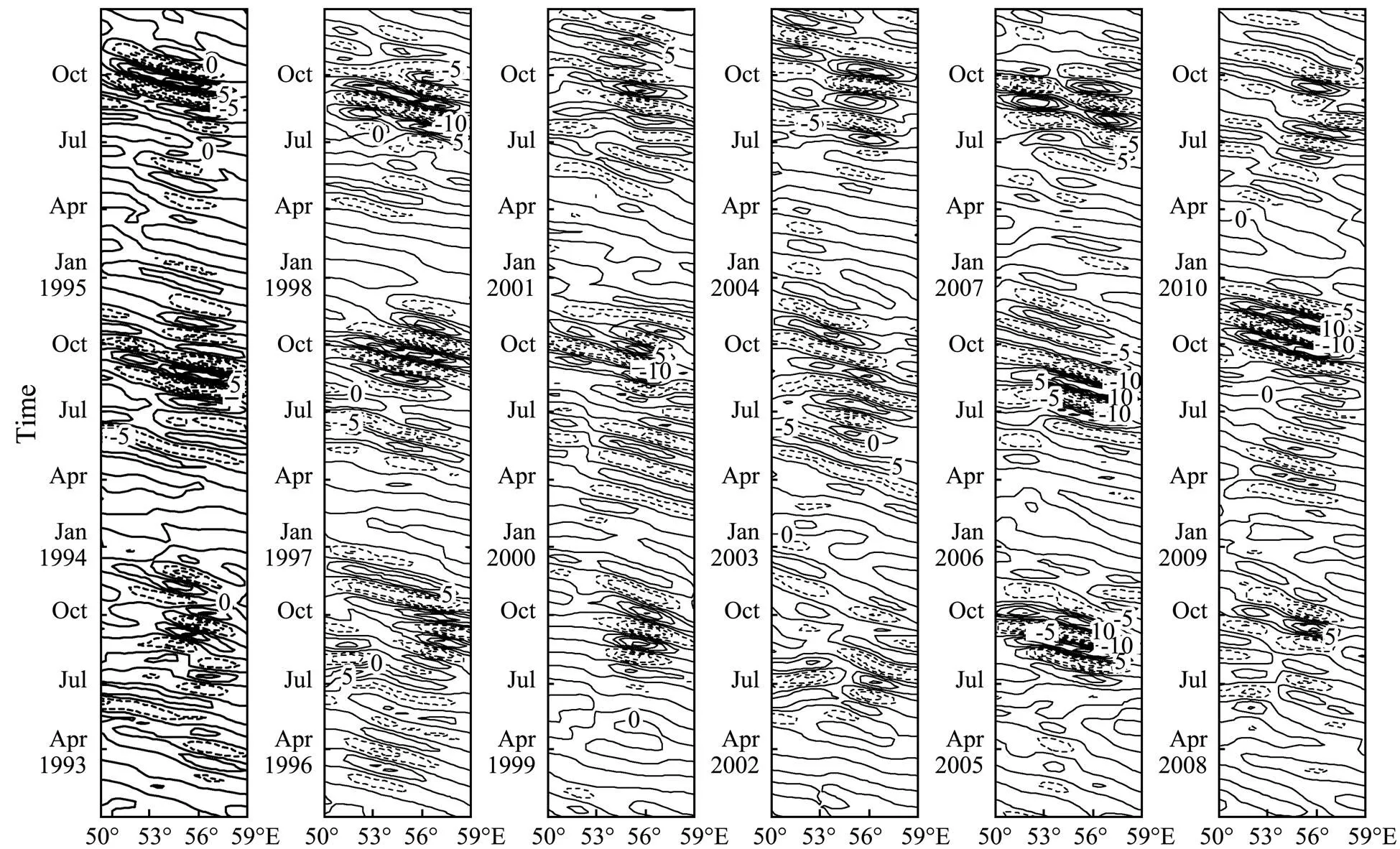
Fig.8 Time-longitude plot of the intraseasonal signals of SLA (cm) along 7.75˚N.
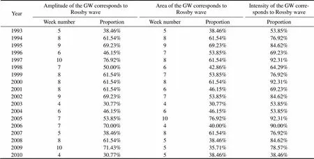
Table 2 Influence of westward propagating Rossby waves on the intensity of the GW
4.3 Relationship Between Ocean Internal Instability and the GW
The intensity of ocean internal instability can be quantified by the barotropic and baroclinic energy conversion rates (Meng, 2006; Yu and Potemra, 2006). The former, however, can not be estimated here due to lack of data. The latter is calculated by the following formula (Meng, 2006; Shore, 2008)

wherek=1000m2s−1andis the gravitational acceleration;is seawater density, which can be obtained from Argo temperature and salinity. This formula indicates that the spatial structure of the density determines the baroclinic energy conversion rate. A larger horizontal density variation and a smaller vertical one will lead to a larger baroclinic energy conversion rate and vice versa.
Fig.9 shows the regional mean baroclinic energy conversion rate as a function of time, averaged over 8˚–12˚N, 51˚–55˚E, and in the depth range of 100–200m. Large values in the year 2005 and 2007 (Fig.9) correspond well to large intensity of the GW in those two years (Fig.2b), implying that more energy can be converted from mean flow into eddy energy, which benefits the generation of the GW. There are two top peaks of the baroclinic energy conversion rate between July and October each year, and the most eastward position in year 2005 (including 2007) corresponds well to the first top peak, while the most westward position in 2003 (Table 1) is in agreement with the second one (Fig.9). The termination time of the GW (Table 1) is also closely related to the baroclinic energy conversion rate (Fig.9). For example, the earliest disappearance of the GW in 2006 and the two very late ones in 2005 and 2007 (Table 1) corresponds well to the earliest and very late occurrences of the second peaks in baroclinic energy conversion rate. This result is consistent with Jensen (1991), who suggests that the eventual decay of the GW is due to baroclinic instability caused by its interaction with an adjacent cyclone, which is generated by shear between the GW and the island of Socotra.
It should be pointed out that none of the wind stress, Rossby wave and baroclinic energy conversion rate could explain all characters of the GW by 100 percent, indicating that the variations of the GW may be caused by the total effect of the atmospheric forcing, Rossby waves and oceanic instability, and so on. However, the relative importance of them is hard to compare quantitatively by the methods used here.
5 Summary
In this paper, AVISO, QuikSCAT and Argo datasets are used to analyze the characteristics of the interannual variability and the related mechanisms of the GW. The main results are as follows:
1) The GW appeared between late April and early June (May 19±22 days) and lasted until around the end of October (October 30±18 days), typically lasting 164±26 days per year, with a center usually located in 52.88˚–53.70˚E, 6.83˚–8.71˚N.
2) The GW appeared earlier (later) in 1993, 2001, 2002, 2004 (in 1994, 1996, 2008) and disappeared earlier (later) in 1993, 1998, 2003, 2006 (in 2001, 2010). The abnormally short (long) duration occurred in 1998, 2006, 2008 (in 2001, 2002, 2004).
3) The GW was located more to the west (east) in 1993, 1999, 2003 (in 1995, 2005) and was more southward (northward) in 1999, 2003, 2007 (in 1995, 1997, 2005).
4) Abnormally strong (weak) years of the GW, determined by amplitude and area, occurred in 1997, 1998, 2005, 2007, 2008, 2009 (in 1994, 1999, 2002, 2003).
5) Preliminary analysis shows that the interannual variability of the GW is closely related to that of intraseasonal wind stress curl in GW region; the generation of the GW is coincident with the arrival of Rossby waves at the Somali coast in spring; the intensity of the GW is also influenced by Rossby waves; the termination time and the intensity of the GW both corresponds well to large baroclinic energy conversion rates in GW region.
Obviously, theoretical analyses and numerical model studies are needed in order to further reveal the dynamical mechanism, including the comparison of the relative importance of different processes.
Acknowledgements
The AVISO data used in this paper are from the French space agency satellite oceanography archive center (http://www.aviso.oceanobs.com/). Argo data are provided by the CoriolisDataCenter,France.QuikSCATdatacanbedownloaded from the website http://www.remss.com/qscat/qscat_browse.html. We are gratefulto the two anonymous reviewersfor many comments and suggestions which helped improve thepaper considerably. This study is supported by the National Natural Science Foundation of China (Grant No. 41076004).
Beal, L. M., and Chereskin, T. K., 2003. The volume transport of the Somali Current during the 1995 southwest monsoon., 50: 2077-2089.
Beal, L. M., and Donohue, K. A., 2013. The Great Whirl: Observations of its seasonal development and interannual variability., 118: 1-13, DOI: 10.1029/2012JC008198.
Brandt, P., Stramma, L., Schott, F., Fischer, J., Dengler, M., and Quadfasel, D., 2002. Annual Rossby waves in the Arabian Sea from TOPEX/POSEIDON altimeter anddata,, 49: 1197-1210.
Bruce, J. G., Fieux, M., and Gonella, J., 1981. A note on the continuance of the Somali eddy after the cessation of the Southwest monsoon., 4: 7-9.
Bunker, A. F., 1976. Computations of surface energy flux and annual air-sea interaction cycle of the North Atlantic Ocean., 104: 1122-1140.
Chaigneau, S., Gizolme, A., and Grados, C., 2008. Mesoscale eddies off Peru in altimeter records: Identification algorithms and eddy spatio-temporal patterns.,79: 106-119.
Chelton, D. B., Schlax, M. G., and Samelon, R. M., 2011. Global observations of nonlinear mesoscale eddies., 91: 167-216.
Chelton, D. B., Schlax, M. G., Samelson, R. M., and de Szoeke, R. A., 2007. Global observations of large oceanic eddies., 34, L15606, DOI: 10.1029/2007GL030812.
Fischer, J., Schott, F., and Stramma, L., 1996. Current and transports of the Great Whirl-Socotra Gyre system during the summer monsoon, August 1993., 101: 3573-3687.
Hu, R. J., and Wei, M., 2013. Intraseasonal oscillation in the global ocean temperature inferred from Argo., 30 (1): 29-40.
Jensen, T. G., 1991. Modeling the seasonal undercurrents in the Somali Current system.,96: 22151-22167.
Li, C. Y., Hu, R. J., and Yang, H., 2005. Intraseasonal oscillation in the tropical Indian Ocean., 22: 617-624.
Luther, M. E., 1999. Interannual variability in the Somali Current 1954–1976., 35: 59-83.
Luther, M. E., and O’Brien, J. J., 1985. A model of the seasonal circulation in the Arabian Sea forced by observed winds., 14: 353-385.
Luther, M. E., and O’Brien, J. J., 1989. Modeling the variability in the Somali Current, in Mesoscale/Synoptic coherent structures in geophysical turbulence., 50: 373-386.
Luther, M. E., O’Brien, J. J., and Meng, A. H., 1985. Morphology of the Somali Current system during the Southwest Monsoon..Nihoul, J. C. J., ed., Amsterdam, Elsevier, 405-437.
McCreary, J. P., and Kundu, P. K., 1988. A numerical investigation of the Somali Current during the Southwest Monsoon., 46: 25-58.
McCreary, J. P., Kundu, P. K., and Molinari, R. L., 1993. A numerical investigation of dynamics, thermodynamics and mixed-layer processes in the Indian Ocean., 31: 181-244.
McCreary, J. P., Kohler, K. E., Hood, R. R., and Olson, D. B., 1996. A four-component ecosystem model of biological activity in the Arabian Sea., 37: 117-165.
Meng, X. F., Wu, D. X., Lin, X. P., and Lan, J., 2006. A further investigation of the decadal variation of ENSO characteristics with instability analysis., 23: 156-164.
Qin, Z. H., 1980. A contribution to the calculation of wind stress on sea surface., 3: 1-8(in Chinese).
Saji, N. H., and Yamagata, T., 2003. Possible impacts of Indian Ocean Dipole mode events on global climate., 25: 151-169.
Schott, F., 1983. Monsoon response of the Somali Current and associated upwelling., 12: 357-381.
Schott, F., and McCreary, J. P., 2001. The monsoon circulation of the Indian Ocean., 51: 1-123.
Schott, F., and Quadfasel, D., 1982. Variability of the Somali current system during the onset of the Southwest Monsoon, 1979., 12: 1343-1479.
Schott, F., Fischer, J., Garternicht, U., and Quadfasel, D., 1997. Summer monsoon response of the northern Somali Current, 1995., 24: 2565-2568.
Shore, J., Stacey, M. W., and Wright, D. G., 2008. Sources of eddy energy simulated by a model of the Northeast Pacific Ocean., 38: 2283-2293.
Tomczak, M., and Godfrey, J. S., 2003. The Coriolis force, geostrophy, Rossby waves and the westward intensification. In:. Daya Publishing House, Delhi, 29–38.
Torrence, C., and Compo, G. P., 1998. A practical guide to wavelet analysis., 79: 61-78.
Weiss, J., 1991. The dynamics of enstrophy transfer in two dimensional hydrodynamics., 48: 273-294, DOI: 10.1016/0167-2789(91)90088-Q.
Wirth, A., Willebrand, J., and Schott, F., 2002. Variability of the Great-Whirl from observations and models., 49: 1279-1295.
Wu, Y. L., Du, Y., Zhang, Y. H., and Zhang, X. T., 2012. Interannual variability of sea surface temperature in the northern Indian Ocean associated with ENSO and IOD., 5 (4): 295-300.
Yu, Z., and Potemra, J., 2006. Generation mechanism for the intraseasonal variability in the Indo-Australian basin., 111: 1-11.
(Edited by Xie Jun)
DOI 10.1007/s11802-015-2392-8
ISSN 1672-5182, 2015 14 (1): 17-26
© Ocean University of China, Science Press and Springer-Verlag Berlin Heidelberg 2015
(May 7, 2013; revised July 23, 2013; accepted October 20, 2014)
* Corresponding author. Tel: 0086-532-66781301 E-mail: huruijin@ouc.edu.cn
 Journal of Ocean University of China2015年1期
- Journal of Ocean University of China的其它文章
- The Influence of El Niño on MJO over the Equatorial Pacific
- Brightness Temperature Model of Sea Foam Layer at L-band
- Parametric Instability Analysis of Deepwater Top-Tensioned Risers Considering Variable Tension Along the Length
- DPOI: Distributed Software System Development Platform for Ocean Information Service
- Nonlinear Contact Between Inner Walls of Deep Sea Pipelines in Buckling Process
- Floating Escherichia coli by Expressing Cyanobacterial Gas Vesicle Genes