
Pressure gradient errors in a covariant method of implementing the σ-coordinate: idealized experiments and geometric analysis
2016-11-23 03:30LIJinXiLIYiYunndWANGBin
LI Jin-XiLI Yi-Yunnd WANG Bin,c
aState Key Laboratory of Numerical Modeling for Atmospheric Sciences and Geophysical Fluid Dynamics, Institute of Atmospheric Physics,Chinese Academy of Sciences, Beijing, China;bCollege of Earth Science, University of Chinese Academy of Sciences, Beijing, China;cMinistry of Education Key Laboratory for Earth System Modeling, and Center for Earth System Science, Tsinghua University, Beijing, China
Pressure gradient errors in a covariant method of implementing the σ-coordinate: idealized experiments and geometric analysis
LI Jin-Xia,bLI Yi-Yuanaand WANG Bina,c
aState Key Laboratory of Numerical Modeling for Atmospheric Sciences and Geophysical Fluid Dynamics, Institute of Atmospheric Physics,Chinese Academy of Sciences, Beijing, China;bCollege of Earth Science, University of Chinese Academy of Sciences, Beijing, China;cMinistry of Education Key Laboratory for Earth System Modeling, and Center for Earth System Science, Tsinghua University, Beijing, China
A new approach is proposed to use the covariant scalar equations of the σ-coordinate (the covariant method), in which the pressure gradient force (PGF) has only one term in each horizontal momentum equation, and the PGF errors are much reduced in the computational space. In addition, the validity of reducing the PGF errors by this covariant method in the computational and physical space over steep terrain is investigated. First, the authors implement a set of idealized experiments of increasing terrain slope to compare the PGF errors of the covariant method and those of the classic method in the computational space. The results demonstrate that the PGF errors of the covariant method are consistently much-reduced, compared to those of the classic method. More importantly, the steeper the terrain, the greater the reduction in the ratio of the PGF errors via the covariant method. Next,the authors use geometric analysis to further investigate the PGF errors in the physical space, and the results illustrates that the PGF of the covariant method equals that of the classic method in the physical space; namely, the covariant method based on the non-orthogonal σ-coordinate cannot reduce the PGF errors in the physical space. However, an orthogonal method can reduce the PGF errors in the physical space. Finally, a set of idealized experiments are carried out to validate the results obtained by the geometric analysis. These results indicate that the covariant method may improve the simulation of variables relevant to pressure, in addition to pressure itself, near steep terrain.
ARTICLE HISTORY
Revised 27 February 2016
Accepted 25 March 2016
Pressure gradient force errors; covariant scalar equations of the σcoordinate; steep terrain;computational and physical space; geometric analysis; non-orthogonal σ-coordinate
本文针对经典σ坐标的气压梯度误差(PGF误差),采用多种地形展开理想试验,对比经典σ坐标的经典方案和协变方案的PGF误差。结果表明:计算空间中,协变方案始终能减小经典方案的误差,地形越陡,效果越明显。然而,几何分析和理想试验均表明:协变方案仅能减小计算空间的误差,不能减小物理空间的误差;相比经典方案,正交地形追随坐标能同时减小计算空间和物理空间的误差。
1. Introduction
The pressure gradient force computational errors (PGF errors) in a terrain-following coordinate (σ-coordinate) can signifcantly afect the performance of a model, including the vorticity in the downslope of steep terrain, the blocking of cold air in the upslope of steep terrain, the potential vorticity near the tropopause over steep terrain, and so on (Smagorinsky et al. 1967; Kasahara 1974; Mahrer 1984;Steppeler et al. 2003; Hoinka and Zängl 2004; Li, Chen, and Shen 2005; Hu and Wang 2007). The PGF computational form is expressed by two terms in each horizontal momentum equation in the σ-coordinate. Computational errors are therefore inevitable as these two terms are opposite in sign and typically of the same order near steep terrain(Haney 1991; Fortunato and Baptista 1996; Lin 1997; Ly and Jiang 1999; Berntsen 2002; Chu and Fan 2003; Shchepetkin and McWilliams 2003; Li, Chen, and Li 2012).
Much efort has been made to alleviate the PGF errors to an acceptable level (Corby, Gilchrist, and Newson 1972;Gary 1973; Zeng 1979; Qian and Zhong 1986; Blumberg and Mellor 1987; Yu 1989; Qian and Zhou 1994; Berntsen 2011; Klemp 2011; Zängl 2012), without touching this twoterm PGF (the so-called classic method). Alternatively, two new methods have been proposed to create a one-term PGF to overcome the PGF errors. One is to adopt the covariant scalar equations of the σ-coordinate (the covariant method by Li, Wang, and Wang (2012)); and the other is to design an orthogonal terrain-following coordinate (the orthogonal method by Li et al. (2014)). Using two idealizedexperiments, Li, Wang, and Wang (2012) showed that the covariant method signifcantly reduces the errors, compared to the classic method, in the computational space.

Figure 1.The pressure feld (shading) and terrain (black curve). The pressure scale (color bar on the right) is in hPa.
Many researchers have pointed out that the PGF errors of the classic method are related to terrain slope (Yan and Qian 1981; Zeng and Ren 1995; Steppeler et al. 2003; Weller and Shahrokhi 2014; Li, Li, and Wang 2016). But can the covariant method consistently reduce the PGF errors compared to the classic method as terrain slope increases?Moreover, although the calculation of a model is in the computational space, the fnal application of model results is in the physical space; can the covariant method reduce the PGF errors in the physical space?
In this study, we frst carry out a set of sensitivity experiments of increasing terrain slope to compare the PGF errors of the classic method and those of the covariant method in the computational space. Then, we use a geometric schematic and associated idealized experiments to further investigate the PGF errors of these methods in the physical space. The results of the idealized experiments using various terrain in the computational space are presented in Section 2. The PGF errors in the physical space are compared in Section 3. Concluding remarks and a discussion are given in Section 4.
2. Idealized experiments in the computational space
Since the covariant method was shown to significantly reduce the PGF errors in the computational space,compared to the classic method, in the experiments using one kind of terrain implemented by Li, Wang, and Wang (2012), we further investigate the PGF errors of the covariant method and those of the classic method in the computational space over different kinds of terrain. We first introduce the basic parameters for all the experiments, and then compare the PGF errors of the covariant method and those of the classic method in the computational space in experiments of increasing terrain slope.
2.1. Basic parameters
For consistency, we use the same parameters as Li, Wang,and Wang (2012), except for the terrain slope. First, the defnition of σ, proposed by Gal-Chen and Somerville (1975) is adopted, where z represents the height, HTis the top of the model, and h represents terrain. We use a 2D bell-shaped terrain (black curve in Figure 1),

where H = 4 km is the maximum height, a = 5 km is the half width, and h0= 50 km is the middle point of the terrain.
Second, we use the centeral spatial discretization for the PGF in the horizontal and the forward scheme in the vertical for both methods. The expressions are given as follows:

Finally, we use a pressure feld,

as shown in Figure 1, where h(x) is defned by Equation (1), H is the maximum height of terrain, Hp= 300 km is a parameter to adjust the pressure gradient, p0= 1,015.0 hPa is surface pressure, and λ = 8 km is the typical height of the atmosphere. The domain of all the experiments is 0-100 km in the horizontal and 0-37 km in the vertical (Figure 1). The horizontal and vertical resolutions are 0.5 km and 3.7 km, respectively.

Figure 2.RMS-REs of two methods in the computational space in experiments of increasing terrain slope. The slope is calculated by arctan (H/2a) and shown in (a). The RMS-REs of each method are shown in (b).
2.2. Sensitivity experiments
Through increasing the maximum height H of terrain in Equation (1) at 50-m intervals from 3 to 9 km, we carry out 121 sets of experiments (Figure 2(a)). Note that the maximum slope is almost three times the minimum in Figure 2(a).
We calculate the root-mean-square of relative errors(RMS-REs) of the PGF of the covariant method and those of the classic method (Figure 2(b)). The RMS-REs of the covariant method are consistently reduced by one order of magnitude, compared to those of the classic method. Moreover, as the terrain slope increases, the RMS-REs of the classic method significantly increase (red line in Figure 2(b) relative to black line in Figure 2(a)); however,the RMS-REs of the covariant method remain approximately the same (blue line in Figure 2(b) relative to black line in Figure 2(a)). Therefore, the steeper the terrain, the greater the reduction of the ratio of PGF errors via the covariant method.
3. Comparison of the PGF errors in the physical space
In order to compare the PGF errors of the covariant method and those of the classic method in the physical space, we frst use a geometric schematic to further investigate the PGF errors in the physical space, and then carry out a set of associated idealized experiments to validate the results obtained by the geometric analysis.
The geometric schematic of PGF is shown in Figure 3. The relationship between the lines with arrow heads in Figure 3 and the variables related to PGF are all listed below:
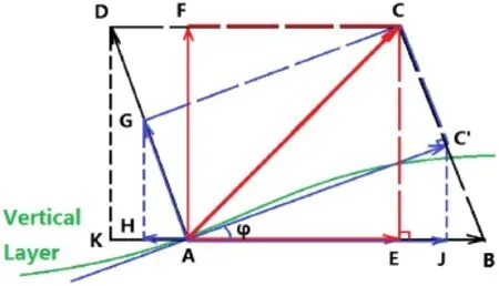
Figure 3.Schematic of PGF vectors and their components in diferent methods.
The vertical PGF of the z-coordinate,

The horizontal PGF of the covariant method in the computational space,The vertical PGF of the covariant method in the computational space,


In addition, through the geometric relationship in Figure 3,we obtain

where φ is terrain slope, and

First, the expressions of the PGF of the covariant method and the classic method in the physical space are respectively given by

According to Equation (7), the PGF of the covariant method expressed in Equation (9) equals the PGF of the classic method shown in Equation (10); namely, the covariant method cannot reduce the PGF errors in the physical space compared to the classic method.
Note that both the classic method and the covariant method are non-orthogonal methods (Li, Wang, and Wang 2011, 2012), namely, the PGF errors in the physical space cannot be reduced by the coordinate transformation in the non-orthogonal σ-coordinate. But can the orthogonal method proposed by Li et al. (2014) reduce the PGF errors in the physical space?

Second, according to Figure 3, the horizontal and vertical PGFs of the orthogonal method in the computational space are respectively, where x′ is the horizontal coordinate of the orthogonal terrain-following coordinate. Then, the PGF of the orthogonal method in the physical space can be expressed by

Using the geometric relationship in Figure 3, we obtain

Substituting Equations (5) and (7) into Equations (14) and(15), we obtain

Note that the PGF of the orthogonal method in the physical space is AJ-AH and that of the non-orthogonal method is AB-BE. According to Equation (16), the PGF errors in the physical space can be reduced by the orthogonal method when the terrain slope φ is large enough:
(1) If is large enough to make the order of AH smaller than that of AJ, i.e. AH and AJ are no longer of the same order, the PGF errors in the physical space can be reduced by the orthogonal method;


Figure 4.REs of three methods in the computational and physical spaces. The dashed contours are for negative values. The contour interval in (a), (b), (d), and (f) is 1.0, while that in (c) and (e) is 0.1. The diferences between (a) and (c) in this study and Li, Wang, and Wang(2012, Figure 6(c) and (d)) on the boundaryare due to the revised boundary condition used in this study. The revised boundary condition is directly from the defnition of pressure , to obtain the value on each boundary grid.


Finally, we calculate the PGF errors of the three methods, i.e. the classic method, the covariant method and the orthogonal method. Substituting Equations (4), (5), (6), (8),(11), and (12) into Equations (9), (10), and (13), and using the discretization schemes given in Section 2.1, we can obtain the discrete expressions of the PGF of the three methods in the physical space as follows:Using Equations (17)-(19) and the parameters given in Section 2.1, we calculate the REs of the PGF of the three methods in the computational space as well as in the physical space (Figure 4). As obtained in the geometric analysis,the PGF errors of the covariant method are the same as those of the classic method in the physical space (Figure 4(b) and(d)), whereas the PGF errors of the orthogonal method are much reduced compared to those of the classic method in the physical space (Figure 4(b) and (f)). In addition, as with the covariant method, the orthogonal method can also reduce the PGF errors of the classic method in the computational space (Figure 4(a), (c), and (e)).
4. Conclusion and discussion
Through idealized experiments using increasing terrain slope in the computational space and a geometric analysis in the physical space, the present study investigates the validity of reducing the PGF errors via the covariant method proposed by Li, Wang, and Wang (2012), compared to the classic method. First, sensitivity experiments of increasing terrain slope in the computational space show that the RMS-REs of the covariant method are consistently one order of magnitude smaller than those of the classic method (Figure 2). More importantly, the steeper the terrain, the greater the reduction in the ratio of PGF errors via the covariant method, indicating that the covariant method may perform better near steep terrain.
The geometric analysis (Figure 3) and associated idealized experiments then demonstrate that, compared to the classic method, the covariant method based on the non-orthogonal σ-coordinate can reduce the PGF errors in the computational space but not in the physical space(Figure 4(a)-(d)). However, the orthogonal method proposed by Li et al. (2014) can reduce the PGF errors in the computational space as well as in the physical space(Figure 4(a) and (b), (e) and (f)).
In addition, since the covariant method cannot reduce the PGF errors in the physical space, but can signifcantly reduce the errors in the computational space, especially over steep terrain, the covariant method may not improve the simulation of pressure itself but could lead to improvement in the velocity (relevant to pressure, according to the momentum equations). For example, Weller and Shahrokhi(2014) used the curl-free PGF (the PGF of the covariant method is curl-free in the computational space) to obtain a better hydrostatic balance and better energy conservation.
Besides, the patterns of PGF error of the orthogonal method are diferent from those of the other two methods based on the non-orthogonal σ-coordinate (Figure 4(a)-(d), (e) and (f)). This is related to the diference between computational grids in the orthogonal σ-coordinate and those in the non-orthogonal σ-coordinate used in this study. Further analyses are needed to investigate the relationship between computational grids and PGF errors. Plus, the true benefts of the covariant method and the orthogonal method need to be tested using primitive equations in more idealized experiments and realistic simulations.
Disclosure statement
No potential confict of interest was reported by the authors.
Funding
This work was jointly supported by the National Basic Research Program of China (973 Program) [grant number 2015CB954102];the National Natural Science Foundation of China [grant number 41305095], [grant number 41175064].
Notes on contributors
LI Jin-Xi is a PhD candidate at LASG, Institute of Atmospheric Physics, Chinese Academy of Sciences. His main research interests focus on dynamical core of atmospheric models. Recent publications include papers in Atmospheric and Oceanic Science Letters, Geoscientifc Model Development, Atmospheric Science Letters, and Chinese Science Bulletin.
LI Yi-Yuan is an associated researcher at LASG, Institute of Atmospheric Physics, Chinese Academy of Sciences. Her main research interests are the numerical methods for the dynamical core of atmospheric models, especially the methods related with the vertical. Recent publications include papers in Geoscientifc Model Development, Communication in Computational Physics,and Atmospheric Science Letters.
WANG Bin is a professor at LASG, Institute of Atmospheric Physics, Chinese Academy of Sciences and CESS, Tsinghua University. His main research interests are the numerical methods and data assimilation for the atmospheric, oceanic, and coupled models. Recent publications include papers in Geoscientifc Model Development, Monthly Weather Review, and Tellus.
References
Berntsen, J. 2002. “Internal pressure errors in sigma-coordinate ocean models.” Journal of Atmospheric and Oceanic Technology 19: 1403-1414. doi:http://dx.doi.org/10.1175/1520-0426(2002)019<1403:IPE ISC>2.0.CO;2.
Berntsen, J. 2011. “A perfectly balanced method for estimating the internal pressure gradients in sigma-coordinate ocean models.” Ocean Modelling 38: 85-95. doi:http://dx.doi. org/10.1016/j.ocemod.2011.02.006.
Blumberg, A. F., and G. L. Mellor. 1987. “A description of a three-dimensional coastal ocean circulation model.”Paper presented at the annual meeting for the American Geophysical Union, Washington, DC, 1-16. doi:http://dx.doi. org/10.1029/CO004p0001.
Chu, P. C., and C. Fan. 2003. “Hydrostatic correction for sigma coordinate ocean models.” Journal of Geophysical Research 108: 3206-3217. doi:http://dx.doi.org/10.1029/2002JC001668.
Corby, G. A., A. Gilchrist, and R. L. Newson. 1972. “A general circulation model of the atmosphere suitable for long period integrations.” Quarterly Journal of the Royal Meteorological Society 98: 809-832. doi:http://dx.doi.org/10.1002/qj.49709841808.
Fortunato, A. B., and A. M. Baptista. 1996. “Evaluation of horizontal gradients in sigma-coordinate shallow water models.” Atmosphere-Ocean 34: 489-514. doi:http://dx.doi.or g/10.1080/07055900.1996.9649574.
Gal-Chen, T., and R. C. J. Somerville. 1975. “On the use of a coordinate transformation for the solution of the Navierstokes equations.” Journal of Computational Physics 17: 209-228. doi:http://dx.doi.org/10.1016/0021-9991(75)90037-6.
Gary, J. M. 1973. “Estimate of truncation error in transformed coordinate, primitive equation atmospheric models.” Journal of the Atmospheric Sciences 30: 223-233. doi:http://dx.doi. org/10.1175/1520-0469(1973)030<0223:EOTEIT>2.0.CO;2.
Haney, R. L. 1991. “On the pressure gradient force over steep topography in sigma coordinate ocean models.” Journal of Physical Oceanography 21: 610-619. doi:http://dx.doi. org/10.1175/1520-0485(1991)021<0610:OTPGFO>2.0.CO;2.
Hoinka, K. P., and G. Zängl. 2004. “The infuence of the vertical coordinate on simulations of a PV streamer crossing the Alps.”Monthly Weather Review 132: 1860-1867. doi:http://dx.doi. org/10.1175/1520-0493(2004)132h1860:TIOTVCi2.0.CO;2.
Hu, J. L., and P. X. Wang. 2007. “The errors of pressure gradient force in high-resolution meso-scale model with terrainfollowing coordinate and its revised scheme.” Chinese Journal of Atmospheric Sciences 31: 109-118 (In Chinese). doi:http:// dx.doi.org/10.3878/j.issn.1006-9895.2007.01.11.
Kasahara, A. 1974. “Various vertical coordinate systems used for numerical weather prediction.” Monthly Weather Review 102: 509-522. doi:http://dx.doi.org/10.1175/1520-0493(1974)102<0509:VVCSUF>2.0.CO;2.
Klemp, J. B. 2011. “A terrain-following coordinate with smoothed coordinate surfaces.” Monthly Weather Review 139: 2163-2169. doi:http://dx.doi.org/10.1175/MWR-D-10-05046.1.
Li, X. L., D. H. Chen, and X. S. Shen. 2005. “Impact study on the calculation of vertical velocity in diferent vertical coordinate.”Journal of Tropical Meteorology 21: 265-276 (In Chinese).
Li, Y. Y., B. Wang, and D. H. Wang. 2011. “Characteristics of a terrain-following sigma coordinate.” Atmospheric and Oceanic Science Letters 4: 157-161. doi:http://dx.doi.org/10.1080/167 42834.2011.11446922.
Li, Chao, D. H. Chen, and X. L. Li. 2012. “A design of heightbased terrain-following coordinates in the atmospheric numerical model: theoretical analysis and idealized tests.”Acta Meteorologica Sinica 70 (6): 1247-1259 (In Chinese).
Li, Y. Y., D. H. Wang, and B. Wang. 2012. “A new approach to implement sigma coordinate in a numerical model.”Communications in Computational Physics 12: 1033-1050. doi:http://dx.doi.org/10.4208/cicp.030311.230911a.
Li, Y. Y., B. Wang, D. H. Wang, and J. X. Li, and L. Dong. 2014.“An orthogonal terrain-following coordinate and its preliminary tests using 2-D idealized advection experiments.”Geoscientifc Model Development 7: 1767-1778. doi:http:// dx.doi.org/10.5194/gmd-7-1-2014.
Li, J. X., Y. Y. Li, and B. Wang. 2016. “Characteristics of Pressure Gradient Force Errors in a Terrain-Following Coordinate.” Atmospheric and Oceanic Science Letters 9(3): 211-218. doi:http://dx.doi.org/10.1080/16742834.2 016.1164570.
Lin, S. J. 1997.“A fnite-volume integration method for computing pressure gradient force in general vertical coordinates.”Quarterly Journal of the Royal Meteorological Society 123: 1749-1762. doi:http://dx.doi.org/10.1002/qj.49712354214.
Ly, L. N., and L. Jiang. 1999. “Horizontal pressure gradient errors of the Monterey bay sigma coordinate ocean model with various grids.” Journal of Oceanography 55: 87-97. doi:http:// dx.doi.org/10.1023/A:1007865223735.
Mahrer, Y. 1984. “An improved numerical approximation of the horizontal gradients in a terrain-following coordinate system.” Monthly Weather Review 112 (5): 918-922. doi:http:// dx.doi.org/10.1175/1520-0493(1984)112<0918:AINAOT>2.0 .CO;2.
Qian, Y. F., and Z. Zhong. 1986. “General forms of dynamic equations for atmosphere in numerical models with topography.” Advances in Atmospheric Sciences 3: 10-22. doi:http://dx.doi.org/10.1007/BF02680042.
Qian, Y. F., and T. J. Zhou. 1994. “Error subtraction method in computing pressure gradient force for high and steep topographic areas.” Journal of Tropical Meteorology 10: 358-368.
Shchepetkin, A. F., and J. C. McWilliams. 2003. “A method for computing horizontal pressure-gradient force in an oceanic model with a nonaligned vertical coordinate.” Journal of Geophysical Research 108: 3090-3123. doi:http://dx.doi. org/10.1029/2001JC001047.
Smagorinsky, J., R. F. Strickler, W. E. Sangster, S. Manabe,J. L. Halloway Jr., and G. D. Hembree. 1967. “Prediction experiments with a general circulation model.” Paper presented at Dynamics of Large Scale Atmospheric Processes,Moscow, USSR, 70-134.
Steppeler, J., R. Hess, U. Schättler, and L. Bonaventura. 2003.“Review of numerical methods for nonhydrostatic weather prediction models.” Meteorology and Atmospheric Physics 82: 287-301. doi:http://dx.doi.org/10.1007/s00703-001-0593-8.
Weller, H., and A. Shahrokhi. 2014. “Curl-Free Pressure Gradients over Orography in a Solution of the Fully Compressible Euler Equations with Implicit Treatment of Acoustic and Gravity Waves.” Monthly Weather Review 142: 4439-4457. doi:http:// dx.doi.org/10.1175/MWR-D-14-00054.1.
Yan, H., and Y. F. Qian. 1981. “On the problems in the coordinate transformation and the calculation of the pressure gradient force in the numerical models with topography.” Chinese Journal of Atmospheric Sciences 5: 175-187. doi:http://dx.doi. org/10.3878/j.issn.1006-9895.1981.02.07.
Yu, R. C. 1989. “Design of the limited area numerical weather prediction model with steep mountains.” Chinese Journal of Atmospheric Sciences 13: 145-158 (In Chinese). doi:http:// dx.doi.org/10.3878/j.issn.1006-9895.1989.02.02.
Zängl, G. 2012. “Extending the numerical stability limit of terrain following coordinate models over steep slopes.”Monthly Weather Review 140: 3722-3733. doi:http://dx.doi. org/10.1175/MWR-D-12-00049.1.
Zeng, Q. C. 1979. “Basic equations and coordinate transformation.” Mathematical and physical fundamental theory for numerical weather prediction. vol. 1, 22-25. Beijing: Science Press.
Zeng, X. P., and Z. H. Ren. 1995. “Quantitative analysis of the discretization errors of the horizontal pressure gradient force over sloping terrain.” Chinese Journal of Atmospheric Sciences 19: 722-732. doi:http://dx.doi.org/10.3878/j.issn.1006-9895.1995.06.09.
气压梯度误差;
协变方案; 陡峭地形; 计算空间和物理空间; 几何分析; 正交地形追随坐标
9 November 2015
CONTACT LI Yi-Yuan liyiyuan@mail.iap.ac.cn
© 2016 The Author(s). Published by Informa UK Limited, trading as Taylor & Francis Group.
This is an Open Access article distributed under the terms of the Creative Commons Attribution License (http://creativecommons.org/licenses/by/4.0/), which permits unrestricted use, distribution, and reproduction in any medium, provided the original work is properly cited.
猜你喜欢
金桥(2022年7期)2022-07-22
数学物理学报(2022年1期)2022-03-16
数学物理学报(2021年6期)2021-12-21
幼儿画刊(2021年5期)2021-12-02
汽车观察(2021年11期)2021-04-24
中学生百科·大语文(2021年2期)2021-03-08
花火彩版A(2021年11期)2021-02-08
应用数学(2020年2期)2020-06-24
装备制造技术(2020年12期)2020-05-22
华东师范大学学报(自然科学版)(2019年3期)2019-06-24
 Atmospheric and Oceanic Science Letters2016年4期
- Atmospheric and Oceanic Science Letters的其它文章
- A decadal abruption of midwinter storm tracks over North Pacific from 1951 to 2010
- Comparison of convective parameterizations in RegCM4 experiments over China with CLM as the land surface model
- Chemical characterization of submicron particles during typical air pollution episodes in spring over Beijing
- Two different periods of high dust weather frequency in northern China
- Biogenic isoprene emissions over China: sensitivity to the CO2inhibition effect
- The link between the Victoria mode in the preceding boreal winter and spring precipitation over the southeastern USA and Gulf of Mexico