
Networked Control Systems:A Survey of Trends and Techniques
2020-02-29 14:12XianMingZhangQingLongHanXiaohuaGeDeruiDingLeiDingDongYueandChenPeng
Xian-Ming Zhang,, Qing-Long Han,, Xiaohua Ge,, Derui Ding,, Lei Ding,, Dong Yue,, and Chen Peng,
Abstract—Networked control systems are spatially distributed systems in which the communication between sensors, actuators,and controllers occurs through a shared band-limited digital communication network. Several advantages of the network architectures include reduced system wiring, plug and play devices,increased system agility, and ease of system diagnosis and maintenance. Consequently, networked control is the current trend for industrial automation and has ever-increasing applications in a wide range of areas, such as smart grids, manufacturing systems,process control, automobiles, automated highway systems, and unmanned aerial vehicles. The modelling, analysis, and control of networked control systems have received considerable attention in the last two decades. The ‘control over networks’ is one of the key research directions for networked control systems. This paper aims at presenting a survey of trends and techniques in networked control systems from the perspective of ‘control over networks’, providing a snapshot of five control issues: sampled-data control, quantization control, networked control, event-triggered control, and security control. Some challenging issues are suggested to direct the future research.
I. INTRODUCTION
THE rapid development of network technologies has brought much change to people’s life. Modern communication networks can provide swift and reliable communication between any two or more physical plants located in different places. Such prominent characteristics make communication networks extensively used to connect control components within a control loop, leading to the so-called networked control systems (NCSs). NCSs have been applied in various areas, such as space exploration, environments, industrial automation, robots, aircraft, automobiles, manufacturing plant monitoring, remote diagnostics and troubleshooting, and teleoperations [1]-[6].
An NCS inherits both advantages and disadvantages from communication networks. On the one hand, communication networks allow data packets to be shared among control components, which means that some traditional point-to-point wiring in the installation of a control system may be avoided.As a result, control cost incurred from installation and maintenance can be reduced significantly. Besides, the wellused communication protocols can ensure data packets to be successfully transmitted between control components, which renders an NCS of high reliability. On the other hand,communication networks transmit data packets only in the form of digital signals rather than continuous signals. This means that signals from physical plants should be sampled and quantized before being transmitted. Moreover, since the network bandwidth is limited, network traffic congestion is unavoidable, usually leading to some constraints such as network-induced delays and packet dropouts. Notice that signal sampling, quantization errors, network-induced delays and packet dropouts may have the effects on control performance of an NCS. Therefore, how to mitigate the effects of those network imperfections on control performance of NCSs has received considerable attention, see, e.g., survey papers [4], [7]-[10] and references therein.
Two of the key research directions for NCSs are ‘control of networks’ and ‘control over networks’ [11]. ‘Control of networks’ aims at providing pretty good quality of service(QoS) of communication networks such that NCSs can achieve satisfactory control performance. In this scenario,network data flows perform very well and network resources can be utilized efficiently and fairly. ‘Control over networks’targets at devising suitable control strategies to reduce the effects of network imperfections on desired control performance. Clearly, ‘control of networks’ focuses on how to improve the QoS of networks while ‘control over networks’on how to enhance control robustness against network constraints. The former is within the field of computer science while the latter falls into the scope of control systems. In this paper, we place emphasis on the latter, i.e., ‘control over networks’.
Recalling the existing literature, a rather large number of results have been reported on ‘control over networks’. Among those results, it is found that more attention is paid to the following five issues:
Sampled-data control, which is to investigate how sampling affects control performance of a control system. Since digital techniques are widely implemented in real-world control systems of continuous-time dynamics, it is more practical that the controller is designed based on sampled data. In a sampled-data control system, one of the fundamental issues to be addressed is how to select a proper sampling period because it directly affects stability of the closed-loop control systems.
Quantization control, which is to study the quantization effects on control systems. The process of converting signals from analog to digital is an example of quantization, which maps input values from a larger set to output values in a smaller set. Quantization can be regarded as a lossy compression procedure. The resultant quantization errors between an input value and its quantized value definitely may deteriorate system performance or destroy system stability.
Networked control, which admits network-induced delays and packet dropouts to exist. Its objective is to investigate the effects of network-induced delays and packet dropouts on control systems. For example, how large is the network-induced delay (or the number of consecutive dropouts) endurable for a control system to retain certain performance? The core issue on such investigations is how to establish a relevant mathematical model for those network-induced constraints. By employing a time-delay system model, an interesting finding is that proper network-induced delays possibly play apositiverole in improving system performance [13].
Event-triggered control, which has become a hot topic since 2007. Under an event-triggered sampling scheme, whether or not to sample system signals is determined by an event rather than the elapse of a fixed period [14]. As a result, computation resources, energy resources and network resources of an NCS can be saved significantly. However, when external disturbances are imposed on the physical plant, the positive minimum inter-event time between any two consecutive sampling instants may not be ensured [15], leading to the socalled Zeno behaviour. In order to elude such Zeno behaviour,a sampled-data-based event-triggered transmission scheme is proposed in [16], which allows system signals to be sampled periodically while an event-generator is used to determine if the sampled signals should be released to the communication network.
Security control, which addresses the security of an NCS in the presence of malicious attacks. Although communication networks provide a convenient platform for wide applications of modern control systems, they are currently vulnerable to malicious attacks due to their openness and insufficient protection. For example, by injecting malicious computer malware, hackers may falsify data packets or change the transmission paths of data packets; and by stealing the encryption key, cyber attackers may illegally get access to the remote control center, resulting in collapse of the control system.Several typical examples about security threats to modern control systems can be referred to Slammer worm on DavisBesse power plant in Ohio, U.S. (2003) [17], Maroochy Shire Council’s sewage control system in Queensland,Australia (2000) [18], and Stuxnet worm which targeted many industrial control systems [19]. Thus, how to detect and cope with attacks such that an NCS works in a safe environment is an important issue, and has been a hot topic in the past decade[20]-[25].
The five control issues above are fundamental issues for NCSs. A great number of notable results have been reported in the literature. This paper presents a survey of trends and techniques in NCSs, focusing on these five issues, and discusses some challenging issues for future research directions.
Notation:P≥0 (respectively,P>0) , wherePis a symmetric matrix, means thatPis positive semi-definite(respectively, positive definite). col{···} represents a blockcolumn vector. N and R are the sets of positive integers and real numbers, respectively.
II. SAMPLED-DATA CONTROL
In a sampled-data system, a continuous-time physical plant is controlled by a digital controller which generates a sequence of control inputs based on the sampled data packets[26]. In the case that the sampling is periodic, there are fruitful and mature results on analysis and synthesis of sampled-data systems, see, e.g., [27], [28]. However, those results may lose their effectiveness when the sampling is aperiodic. Therefore,during the past two decades, aperiodic sampled-data systems have been an active topic in the field of control, and a number of results have been reported in the literature, see, e.g., survey papers [29], [30] and references therein.
Consider the following linear sampled-data system described by

wherex(t) is the system state andu(t) is the control input;AandBare known real matrices of compatible dimensions whileFis the control gain to be designed. An input delay method is well used to analyze stability of the system (1) and design the control gainF. The basic idea is to introduce an artificial piecewise-continuous delay τ(t)=t-tk. Then the control inputu(t) can be rewritten as

which leads to the following time-delay system model of the closed-loop system


By choosing a Lyapunov-Krasovskii functional candidate aswith

whereP>0 andR>0, some criteria on stability and the existence of suitable control gainFare formulated based onLypunov-Krasovskii stability theorem. However, those criteria are conservative [31] since they should be satisfied foranycontinuous delaywhich is a constraintstricterthan (4). Inspired by [32], an improved input delay method for sampled-data systems is proposed in [33], where atime-dependent Lyapunov functionalis constructed asV2(t) =xT(t)Px(t)+VU(t)with

whereU>0. A characteristic ofV2(t) is that it does not grow after the sampling times due to the fact thatVU(t)>0 while it vanishes after the sampling timestk(k=1,2,···). A stabilitytionalasV3(t)=xT(t)Px(t)+VW(t) with [34]theorem tailored for such kinds of time-dependent Lyapunov functionals is also established in [33]. The stability theorem also allows one to construct adiscontinuous Lyapunov func-

whereW>0 andtk≤t<tk+1(k=0,1,2,···). The extended Wirtinger inequality ensures thatVW(t)≥0.
Stability analysis based on the time-independent Lyapunov functionalVR(t), the time-dependent Lyapunov functionalVU(t) and the discontinuous Lyapunov functionalVW(t) can be referred to [34] in detail. It can be found through simulation that a stability criterion based onVU(t) produces a larger upper bound ofh¯ than a stability criterion based on eitherVW(t) orVR(t). A natural question is why the discontinuous Lyapunov functionalVW(t) is introduced. To answer this question, in [34], a sampled-data system is considered by introducing a constant transmission delay into the control inputu(t) , i.e.,u(t)=Fx(tk-η) , where η >0 is a constant. For such a sampled-data system with a positive constant transmission delay, it is shown that the corresponding time-dependent Lyapunov functionalVU(t) bringsno clear advantagesover the correspondingVR(t) (see Remark 1 in[34]), while the discontinuous Lyapunov functionalVW(t) ispreferablesince it can deliver less conservative and simpler results than the other Lyapunov functionalsVR(t) andVU(t).However, from Example 1 in [34], one can see that the obtained results using the discontinuous Lyapunov functional are still conservative. Moreover, it is also illustrated that, by introducing a constant transmission delay into the control input, the upper bound ofis decreased significantly, which reveals thenegative effectsof transmission delays on stability of sampled-data systems.
In 2012, a framework was proposed for stability analysis of sampled-data systems [35]. In this framework, the closed-loop system of the sampled-data system (1) is re-formulated,inspired by the lifting modeling technique. Denote
whereandare two positive constants satisfyingThen for ∀t∈[tk,tk+1), one has thatx(t)=Γ(t-tk)x(tk), where


Let σ:=t-tk∈[0,Tk]. Define a functionχk(σ):=x(tk+σ)(k=1,2,···) . Then χk(σ)=Γ(σ)χk(0), and χk(σ) satisfies

It is clear that the function χk(σ)(σ ∈[0,Tk]) is the state trajectory of the sampled-data system on [tk,tk+1). The first equation in (9) presents the relationship betweenx(tk) andx(tk+1),state trajectory over the period [tk,tk+1). Therefore, the continuous-time method can be employed to investigate the stability of the sampled-data system. Theequivalencebetween discrete-time and continuous-time stability analysis methods is disclosed in [35]. Thesignificanceof the equivalence theorem is that the positive definiteness of the time-dependent Lyapunov functionals and discontinuous Lyapunov functionals can be relaxed by alooping condition. According to this equivalence theorem, a Lyapunov functional candidate can be constructed asV4(t)=xT(t)Px(t)+V0(σ,χk) , whereK →Ris a continuous and differentiable functional satisfying which permits the use of the discrete-time stability analysis method. The second equation in (9) reflects the motion of the

which is a looping condition. In this sense, V0(σ,χk) is called alooped functional. A looped functional suggested in [35] is given as

where ξk(σ)=χk(σ)-χk(0). SinceV0(0,χk)=V0(Tk,χk)holds for, the functional V0(σ,χk) satisfies the looping condition (10) while the real matricesS1,S2,XandRarenotnecessarily positive definite. Revert V0(σ,χk) to a function on timetto obtain

By taking such a looped functional, some less conservative stability conditions are derived in [35]. Borrowing the above idea, atwo-sidedlooped functional is introduced in [36] in the sense that information on both states at two vertices of the interval [tk,tk+1), i.e.x(tk) andx(tk+1), is exploited. It reads asV5(t)=xT(t)Px(t)+V(t), where

with D :=diag{(tk+1-t)I, (t-tk)I} and


III. QUANTIZATION CONTROL
Signals should be coded via analog-to-digital coders before the signals are released to a communication network. On the one hand, an analog-to-digital coder is usually employed to convert a continuous-time analog signal to its corresponding discrete-time digital one [38]. The error between the actual analog value and the converted digital one is usually unavoidable due mainly to the operation of rounding or truncation. On the other hand, data compression of sampled signals is quite common in order to reduce network loads such that limited channel bandwidth can be utilized effectively. As typical coders, quantizers have gained ever-increasing interest of researchers. Essentially, a quantizer is a symmetrical piecewise function with respect to the origin, mapping input values to output values with an infinite countable number of levels [39]. Generally, there areuniform quantizersand
logarithmic quantizers.
Denote a quantizer asf(·) and the number of quantization levels as ♯g(ε) over the interval [ ε, 1/ε]. Its density is defined as [39], [40]

With this definition, a logarithmical increase of the number of quantization levels occurs if the length of interval [ ε, 1/ε] gets larger. A small value of ηfcorresponds to a coarse quantizer.Especially, ηfbecomes zero if the number of quantization levels is finite, while ηfequals infinity if the quantizer is linear. A classical approach to investigating quantization effects is to treat the quantization errors as unknown but bounded disturbance or norm bounded uncertainties. In doing so, classical robustness analysis tools or bounded stability theory can be employed to address various quantization-induced issues. Furthermore, the desired system performance can be guaranteed by adjusting the error bound or the quantization density, and the desired controller or filter parameters can be obtained simultaneously.
A. Uniform Quantizer
Suppose that the overall quantizer range is [-L,L] withL>0. Denote by M the quantizer level length.Letwhere b is the number of bits for digital sensors.Then the uniform quantizer is given by [41]

wheref(y) is the quantized signal andqkis the quantization error process. The quantization error processqkis usually modeled as an unknown but bounded disturbance or an additive white uniform distributed noise with each element being uniformly distributed over [-0.5M, 0.5M]. For a stochastic model, the variance of such a quantization error process is(M2/12)I.
The quantization effect is investigated in [42] with the model above for systems with time-varying delays and input saturation. Both the domain of attraction and the reachable ellipsoid are derived by using a Lyapunov-Krasovskii functional method. It should be pointed out that the obtained reachable ellipsoid is dependent on the quantization error bound 0.5M. Recently, some quantized control issues are addressed by using different control approaches. For example,networked nonlinear systems subject to the try-once-discard protocol scheduling are analyzed in the framework of exponentially ultimate boundedness [43]. Uncertain nonlinear systems subject to input constraints are investigated in the framework of approximate dynamic programming [44].Moreover, a robust analysis method is developed in the case of imprecise quantizer level length [45]. For consensus control of multi-agent systems, there are a number of preliminary results available in the literature, see, e.g., [46], [47] and references therein.
Dynamic quantizers can be employed to guarantee desired closed-loop system performance. A dynamic quantier is based on a dynamic quantizer functionfµ(y)=µf(y/µ), where µ is a dynamic variable referred to as a “zoom” variable, andfis a certain quantizer. The zoom variable µ is used to adjust both the quantizer range and the quantizer error bound based on the value of output measurementy. The simplified form of a dynamic quantizer is described by [48]-[50]

where δµ is the maximum quantization error for allyin the range of the quantizer. Based on the dynamic quantizer above,event-triggered input-to-state stability with a size-adjustable set is investigated in [50]. Moreover, by introducing an adjustable “center” and some “zoom” parameters, a coarse quantizer is studied in [51] to achieve the input-to-state stability with respect to external disturbance. However, when communication protocols are involved, investigating the quantization effects on NCSs becomes more complex and deserves further effort [52]-[54].
B. Logarithmic Quantizer
For the predetermined set of quantization levels

with 0 <ρ ≤1 andu0>0, a logarithmic quantizerf(·) is described by [40], [55]
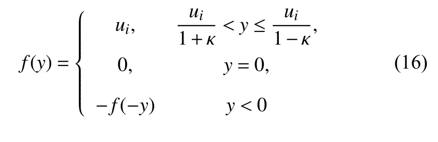
with κ =(1-ρ)/(1+ρ). For such a logarithmic quantizer, it is not difficult to verify that its quantization density satisfies ηf=2/ln(1/ρ). In this sense, the quantized measurement is modeled as

where △ (k)∈[-κ, κ].
There are three kinds of methods to analyze the system performance under a logarithmic quantizer. The first method is based on a quantization-dependent Lyapunov function [55],[56]. Using this method, the obtained conditions depend closely on the parameter κ, leading to some less conservative results on control performance. The second one is called a robust analysis method. If one definesF(k)=κ-1△(k), thenF(k) is an unknown real-valued time-varying matrixF(k)satisfyingFT(k)F(k)≤I. Thus, the quantization control problem can be transformed into the well-known robust control/filtering problem [57], [58]. Based on the robust analysis method, a scheme with the form of coupled recursive Riccati difference equations is developed in [58] to deal with theH∞control of time-varying systems over finite-horizon. It is worth mentioning that this method is similar to the direct utilization of the constraint ‖△(k)‖≤κ, as is done in [59] for recursive filtering. The third method is related to the sector representation of the quantization error of a logarithmic quantizer. The quantization errorqk(y) can also be characterized by the following sector condition

Then the quantized measurement is rewritten as

Some well-known control methods using the above sector condition can be employed to cope with the problem of quantization control, see, e.g., [60] and [61] in detail.
The analysis above just takes a snapshot for quantization control, including two quantizer models and research methods. Some other complex quantization models are not involved in this paper. For example, a logarithmic-hysteretic quantizer is proposed in [62] to describe both the quantization and the deadzone. A logarithmic-uniform quantizer and a hysteresis-uniform quantizer are designed in [63], where a stability analysis approach is developed by constructing a compensation scheme for the effects of the state quantization,and the system performance can be improved by appropriately adjusting design parameters.
IV. NETWORKED CONTROL
In an NCS, sensor data and control signals are transmitted via communication channels from Sensor to Controller (S-C)and from Controller to Actuator (C-A). Due to the limitation of network bandwidth, there exist inevitable network traffic and congestion, thus causing some network-induced phenomena during data transmission. Network-induced delays and packet dropouts are two common phenomena that an NCS encounters, and they are usually regarded as a factor that may degrade system performance or jeopardize the system stability. Thus, how to deal with network-induced delays and packet dropouts has been a fundamental issue, and a great number of results on this topic have been published in the literature, see some monographs [64], [65] and survey papers[4], [7]-[9], [66], [67].
In this section, we present a review of two common models of network-induced delays and packet dropouts, namelyrandom modelandinput delay model, depending on the random and time-varying characteristics of network-induced delays and packet dropouts.
A. Random Model
A random model of network-induced delays and packet dropouts is quite often and natural. This model is usually based on the discrete-time description of the physical plant.Suppose that the S-C and C-A channels have different random attributions. A random model for network-induced delays is established in [68]. Let τk∈[0,τ] anddk∈[0,d] be the random time delays in the S-C channel and the C-A channel,respectively, where τ anddare two known positive integers.A reasonable assumption is made in [68] that two random sequences {τk} and {dk} are homogeneous Markov chains that take values in {0,1,···,τ} and {0,1,···,d} with transition probability matrices [λij] and [πrs], respectively. Under such an assumption, the controller is of the form

It is claimed that the model above of network-induced delays takes packet dropouts into account if λi j=0 or πrs=0 occurs forj>i+1ors>r+1. The advantage of the model above is that the control gainFis not a constant real matrix but a variable one dependent on network-induced delays τkanddk-1.
In [69], [70], random delays in both S-C and C-A channels are modeled as a linear function of a stochastic variable satisfying Bernoulli random binary distribution. Suppose that δ ∈R is a stochastic variable being a Bernoulli distributed white sequence with Prob{δ=1}=and Prob{δ=0}=1-δ¯.The following description of sensor measurementyc,k
provides a random model of network-induced delays, wherexkandykare the system state and the system output, respectively; andCis a constant real matrix. The outputykis sent to an observer subject to the network-induced delay τd. If τdis less than one sampling period,yc,k=yk. If τdis longer than one sampling period but less than two sampling periods,yc,k=yk-1. If δ takes the value of 1 during more than two consecutive sampling periods, it is true that τdis longer than two sampling periods.
The idea above is used to model random packet dropouts[71]. In the S-C channel, let the stochastic variable αk∈R be a Bernoulli distributed white sequence. Then the measurement outputykis described by


wherewkis the disturbance input, andCandDare constant real matrices. αk=0 means that a packet dropout occurs. This measurement outputykis sent to an observer-based controller to generate control signal. Then the control signalis transmitted to actuator via the C-A channel. The random packet dropout phenomenon in the C-A channel is modeled as a stochastic variable βk∈R, which is mutually independent of αk. The stochastic variable βkis also a Bernoulli distributed white sequence. Then the control inputukto actuate the physical plant is given asIf βk=0, thenuk=0, which means that the packet is lost during transmission.
Note that the model (21) is available just for random network-induced delays while the model (22) just for random packet dropouts. A unified model to describe both random network-induced delays and packet dropouts is presented in[72]. The idea is to introduce a number of indicator functionsand(j=1,2,···,q), whereskis a stochastic variable to determine how large the network-induced dela y and the possibility of data missing could be at the time instantk. The stochastic variableskis no longer a Bernoulli distributed white sequence, while its mathematical expectation satisfiesp0and=Prob{sk=dj}=pjwith

Based on this model, if

The analysis above provides several typical stochastic methods to model random network-induced delays and packet dropouts. Although there are different approaches reported in the literature to dealing with the same problem, the basic ideas of them are similar to the ones mentioned above. In the recent years, these methods have stirred up much interest of researchers in the field and have been widely used to handle a number of issues, such as input-to-state stability, input-output stability,H∞control, Kalman filtering,H∞filtering, faulttolerant control and so on.
B. Input Delay Model
An input delay model is well-used to deal with networkinduced delays and packet dropouts. Suppose that the controller and actuator are event-driven while the sensor is time-driven with a periodTs>0. Each sampled signal from the sensor is stamped by time, and encapsulated together with its time-stamp into a packet, say (j,x(jTs))(j=1,2,···). The packet (j,x(jTs)) is transmitted to the controller via the S-C channel and ultimately to the actuator via the C-A channel. If the transmission is successful, the time-consuming denoted by τjfrom the sensor to the actuator is called a network-induced delay, which is lumped together from both channels. Thus, the time-instant when the packet arrives at the actuator can be calculated asjTs+τj. At this time, if state feedback is concerned, the control input that actuates the physical plant can be given by


Fig. 1. The diagram of time scheduling.
This control input will be changed only when the next new packet arrives at the actuator. Since τjis not necessarily equal to τqforthe next new packet transmitted successfully may be not (j+1,x((j+1)Ts)). Denote by {i1,i2,i3,···} the time-stamp sequence indicating that those sampled packets arrive at the actuatorin order. Then it is possible thatik>ik+1,but it must be true thatFig. 1 is an example to show the time-stamp sequence {i1,i2,i3,···}. That is,i1=1,i2=3,i3=4,i4=6,i5=2 andi6=7 . Clearly,i4>i5whileTherefore, the control input can be described by

Define a piecewise continuous function

Then the control inputu(t) can be rewritten as

It is clear that τ(t) includes information on network-induced delays. Moreover, information on packet dropouts is also included in τ(t). In fact, if {i1,i2,i3,···}N, then those packets whose time-stamps belong to the complement set of{i1,i2,i3,···}are dropped out; otherwise, no packet dropouts happen. This model τ(t) has been widely used in NCSs, which is referred to as aninput delay method[73], [74].

Another model can be referred to [76]. The basic idea behind this model is based on the assumption that the properties of both two delays from the S-C channel and the CA channel may not be identical. Denote byds(t) andda(t),respectively, the time-varying delays induced from the S-C channel and the C-A channel. Two network-induced delaysds(t) andda(t) maynotbe combined together since they are of different properties (for instance, one is differentiable while one is non-differentiable). In this situation, the control input(for state feedback) can be described as

Then the closed-loop NCS is modeled as a system withtwo additive time-varying delay components. Although plenty of results on NCSs have been obtained based on this model, how these two delays reflect some exact features of communication networks has not been discussed yet.
The input delay model above has animplicitassumption that there are only one sensor, one controller and one activator in the NCS with no competition of them when gaining access to networks. If there are more network nodes and only one node per transmission is allowed to transmit its packet at any time, proper communication scheduling (or communication protocol) among the nodes is necessary. Arguably, there are two communication protocols available: static and dynamic. A static communication protocol, like Round-Robin (RR),periodically assigns one nodein a prefixed orderto transmit its packet, while a dynamic communication protocol, like Try-Once-Discard (TOD), dynamically assigns one node to transmit its packet based on thenetwork-induced errors[77].Under either an RR protocol or a TOD protocol, it is still challenging to establish such an input delay model as above to handle network-induced delays and packet dropouts simultaneously. For this reason, in [77], it is assumed that no network-induced delays and packet dropouts occur, and in[78], [79], network-induced delays are allowed while packet dropouts are not expected when RR protocols or TOD protocols are involved.
The random and input delay models aforementioned are commonly used to describe both network-induced delays and packet dropouts. Based on these two models, the related closed-loop NCS is modeled as a number of systems either in the continuous-time domain or in the discrete-time domain,such as stochastic systems, time-delay systems, switched systems, Markov jumping systems, impulsive systems, and hybrid systems, and thus leading to a large number of results on NCSs in the open literature. Although those results may reveal more or less effects of network imperfections on NCSs,there is much room for improvement. How to build an exact mathematical model for network imperfections, especially for packet dropouts, such that the effects of them on NCSs can be disclosed explicitly is of much significance and importance both in theory and in practice.
V. EVENT-TRIGGERED CONTROL
Event-triggered control has been long in existence, which can date back to 1960 for the research of an accelerometer with pulse feedback [80], wherepulse generatorsare used to move a pendulum towards the center position once a deviation is detected. Such pulse generators embrace the basic idea of event-triggered control. In 1993, it was pointed out that‘control is not executed unless it is required’ when answering the question ‘Should responsive systems be event-triggered or time-triggered?’ [81]. Unfortunately, this idea did not attract much research interest at that time. Seemingly, it is pretty simple and natural, but its theoretical analysis is quite complicated. An encouraging result contributes to the experimental analysis on a first-order stochastic system, which shows that event-triggered control has a number of advantages compared to time-triggered control [82]. However, the study on event-triggered control is still sporadic until a general solution to the problem of stability is derived for eventtriggered control systems [14]. Boosted by the results, eventtriggered control has been a quite hot topic in the field of NCSs even up until now, see, e.g., survey papers [83]-[85]and references therein.
Event-triggered control is a natural way in the sense that a control execution depends on an event rather than the elapse of a fixed time period. An event-generator is used to detect if an event is triggered before control executes. In an NCS, the event-generator is usually embedded into the sensor to decide whether or not the current signal should be sampled, leading toevent-triggered sampling(Fig. 2(a) ). Alternatively, an event-generator is located behind a sensor to determine if sampled signals should be released to the communication network to transmit, resulting inevent-triggered transmission(Fig. 2(b)). Event-triggered sampling is an ideal approach to choosing only necessarily sampled signals to carry out some desired control tasks such that communication resources,energy resources for battery-based devices, and network resources can be saved to a maximum extent. Nevertheless,event-triggered sampling is liable to fall into Zeno behaviour,which means that infinite sampling times occur within a certain finite time-interval, especially when the system is disturbed by external noises. Event-triggered transmission,however, is based on either periodically or aperiodically sampled data, and thus the Zeno behaviour is not involved. In this sense, such an event-triggered transmission scheme is also known as a sampled-data-based event-triggered transmission scheme [86]-[91], which aims at reducing network loads to save precious network communication resources. It is noteworthy that the sampled-data-based event-triggered transmission scheme can save precious network resources while computation burdens and energy consuming of sensors may not be reduced [30]. In the recent years, event-triggered sampling and event-triggered transmission both have received much attention. The key point is how to devise a suitable condition to generate an event. In this section, we provide a brief summary of recent developments on devising eventtriggering schemes (ETSs) for both event-triggered sampling and event-triggered transmission.
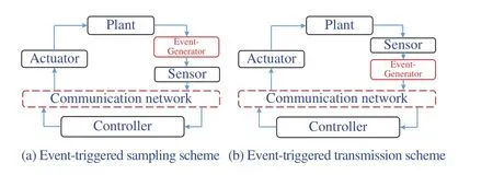
Fig. 2. Two schemes of event-triggered control.
A. ETSs for Event-triggered Sampling
An ETS is originally motivated by Lyapunov stability.Consider the control system described by

wherex(t) andu(t), respectively, are the system state and the control input, respectively. A suitable controlleru(t)=µ(x(t))is designeda priorisuch that the resultant closed-loop system

is input-to-state stable (ISS) with respect toe, whereeis the error vector. Then there exists an ISS Lyapunov functionV(x)satisfying
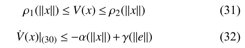
where ρ1(·),ρ2(·),α(·) and γ(·) are class K∞functions1A function α(·) is said to be of class K∞ if it is continuous, strictly increasing and satisfies l ims→∞α(s)=∞ and α (0)=0..
Event-triggered sampling aims to provide a scheme to sample the system state such thatfor allt≥0, whereis a class K∞function. We denote the sampling sequence by

Thenx(t)=x(tk) fortk≤t<tk+1. Sete(t)=x(t)-x(tk),
t∈[tk,tk+1). Suppose that the communication network has ideal quality of service. Then the control input can be given by

In order to maintain the system stability, an event-triggering condition can be devised as

where the threshold σ ∈(0,1) is a constant. Once the condition (35) is satisfied, an event, i.e., sampling the system state,is immediately invoked. In this sense, the sampling instant can be determined by

Such an ETS can deduce the following inequality

which ensures the stability of the closed-loop system under the sampling scheme due to σ ∈(0,1).
The event-triggering condition (35) depends on the system statex(t) and its errore(t) rather than a fixed time period.Thus, signals are sampled only when necessary. In what follows, we give a detailed explanation about the condition.
First, note that α(·) and γ(·) are continuous and strictly increasing functions, and thate(tk)=0 . Hence, attk, one has σα(‖x(tk)‖)>γ(‖e(tk)‖)=0 . According to continuity, whentis increasing fromtk, the inequalityσα(‖x(t)‖)>γ(‖e(t)‖)holds. Second, if the closed-loop system is deviating from its stability,x(t) will be getting larger, leading to the increase of both σα(‖x(t)‖) and γ(‖e(t)‖). Once σα(‖x(t)‖)=γ(‖e(t)‖) is satisfied, a new event timetk+1is generated such thate(t)returns to zero, i.e.e(t)|t=tk+1=0, which turns the closed-loop system back to stability, see Fig. 3.
The ETS above is known as astaticETS. To relax the event-triggering condition (35), adynamicETS is proposed in[92]. The basic idea is to introduce an internal dynamic variable η (t) in (35) such that
where θ >0 is a parameter to be designed, and η (t) satisfies
where β(·) is a class K∞function and η0>0.
Under the dynamic ETS (38), it is proven that η(t)≥0 fort≥0. Attk, σα(‖x(tk)‖)>γ(‖e(tk)‖)=0. Lettincrease slowly fromtk. Then σ α(‖x(t)‖)>γ(‖e(t)‖). Onceσα(‖x(t)‖)=γ(‖e(t)‖)is satisfied, the dynamic ETS (38) allowstto keep going until(38) holds, which means that the inequalityσα(‖x(t)‖)≥γ(‖e(t)‖) does not need to be always satisfied fort≥0. In this sense, the minimum inter-event time min{tk+1-tk|k=0,1,2,···}is larger than that of the static ETS (35). On the other hand, if rewriting (38) as

the dynamic ETS reduces to the static ETS (35) if θ →∞.Such a dynamic ETS is refined in [93] to deal with the distributed set-membership estimation issue for a class of discretetime linear time-varying systems over a wireless multi-sensor network. It is analytically and numerically shown that such a dynamic ETS can lead to larger average inter-event time and thus less totally released data packets.
Note that both the static ETS (36) and the dynamic ETS(38) cannot guarantee a positive minimum inter-event time to avoid Zeno behaviour, especially for perturbed physical plants[15]. In this situation, a mixed time- and event-triggered scheme is proposed in [94], where the sampling instant is calculated by

Fig. 3. Two schemes of event-triggered control.


withT>0 denoting a constant and F(σ,x,e) representing a certain function with respect to σ,xande. Clearly, with this scheme, a positive minimum inter-event time greater thanTis guaranteed even though external disturbance is imposed on the system. This scheme is also studied in [95] by presenting a switching model for the closed-loop system. Mixed time- and event-triggered schemes have strong application background.In fact, in non-rush hours, such a mixed triggering scheme can be used to control the traffic lights’ change. Once a car arrives just before a stopping line, an event should be triggered to turn the light from red to green. Such a task can be completed within a fixed timeTafter the event is triggered.
A common feature of the ETSs above is that the system statex(t) should be monitored at any time. To carry out such a task, extra hardware should be embedded into the system such that an ETS works well. This definitely incurs an increase of cost. In this situation, self-triggered control comes to the fore[96]. The concept of self-trigger means that the next sampling time can bepredictedby the current sampled signal, which can be generally described by

where F(x(tk)) is a prediction function with respect tox(tk). It is clear that a self triggering scheme allows us to compute the next timetk+1offlinebased on the available statex(tk).However, how to define an exact prediction function is a challenging issue. Based on an ISS Lypunov function and L2gain performance, a prediction function is defined as [96]
where α,δ,α,ρ(·) and µ0(·) are referred to [96]. For exponential ISS, a different prediction function is designed in [97].
ETSs for event-triggered sampling have gained considerable attention during the past decade. A large number of results have been reported on ETSs for linear or nonlinear or stochastic systems in either continuous-time or discrete-time domain, see some recent results, e.g., [98]-[106]. However,most results are derived from the digital implementation perspective. First, design a suitable controller such that the closed-loop system has some proper performance. Then,design an ETS to implement the predesigned controller in a digital platform such that the closed-loop performance can be retained while the number of sampling can be reduced as much as possible. This represents a kind ofpassiveeventtriggered control schemes since the ETS should cater for the predesigned controller.Activeevent-triggered control is to actively design a suitable controller for the physical plant under a certain ETS. That is, the controller is designed to cater for the ETS. As such, some closed-loop performance can be ensured while the number of sampling and/or transmission can be reduced to the minimum extent. Nevertheless, such anactiveevent-triggered control scheme remains challenging although is of great practical significance. Another point is that event-triggered control should take communication constraints like network-induced delays and packet dropouts into account, while just few results on them are reported, see,e.g., [99], [100].
B. ETSs for Event-triggered TransmissionAn ETS for event-triggered transmission aims at saving precious network resources by reducing the number of data packets before being released to a communication network. It works at every sampling instant to choose necessary data packets to transmit through networks. Suppose that the sequence of sampling instants is {ih|i=1,2,···}, whereh>0 is the sampling period. The event-triggering condition for an ETS is usually devised as follows [16]

where ε ∈(0,1) is a threshold and Ω a weighting symmetric positive definite matrix; andtkhis the latest time instant when a data-packet is triggered. Based on this condition, the next time instanttk+1hcan be determined by

Analysis in depth on the ETS (44) can be found in [84]. As a complementary, we present one more insight to the condition (43) compared with (35) and (38). A clear observation on the event-triggering conditions (35) and (38) is that they are closely dependent on the derivative of a certain Lyapunov function. This is because they should be designed to passively cater for some preset closed-loop performance.However, the condition (43) is independent of any Lyapunov function and its derivative. The objective of (43) is to reduce the number of sampled data packets. According to the realtime status of network traffic, one can adjust the threshold to release more or less data packets to the network. Then, based on the ETS, we actively design suitable controllers such that the closed-loop system can achieve some expected performance. In this sense, the condition (43) is more practical than those (35) and (38). Thus, it has been widely used to deal with a number of control issues over networks, such asH∞control, L2control, sliding mode control, fuzzy control,adaptive control, stochastic control, distributed control, fault diagnosis, state estimation and filtering, consensus and formation control.
Recently, the event-triggering condition (43) is modified as

where Ω1and Ω2are two different weighting symmetric positive definite matrices [107], [108]. The introduction of the weighting matrix Ω in (43) is just to enhance the feasibility of related linear matrix inequalities [109]. If Ω1and Ω2are two design parameters, then for any threshold ε ∈(0,1), the ETS may be reduced to a time-triggering scheme since there may exist Ω1and Ω2such that no event will be triggered. Thus, the event-triggering condition (45) works well unless Ω1andΩ2are givena priori. Moreover, from some simulation results,we find that the ETS indeed can be regarded as a time-triggering scheme if we setHowever, this finding has not been proven from theoretical points.
The ETSs for both event-triggered sampling and eventtriggered transmission mentioned above are designed based on a constant threshold parameter σ or ε. As a matter a fact, the choice of such a threshold parameter greatly affects a data transmission rate, which is in general time-varying, through practical communication channels. For example, raw transmission rates over an IEEE 802.11b wireless local area network may vary over time at 1, 2, 5.5, and 11 Mb/s due to time-varying interference and random wireless fading [110]. It is thus reasonable to consider an essentially time-varying threshold parameter within ETSs. In [110], by assuming that the threshold parameter in the ETS is time-varying with attainable upper and lower bounds, the problem of distributed event-triggeredH∞consensus filtering for a discrete-time linear system over a wireless sensor network is addressed through a threshold-parameter-dependent approach. Although such an ETS provides certain freedom to adjust the inter-event times, it does not fully explore the relationship between the time-varying threshold parameter and the variant transmission rates over wireless transmission channels, which leaves much room for improvement. Recently, in the context of multi-agent coordination control, for theith agent, a dynamical ETS is proposed as [111]

VI. SECURITY CONTROL
The ever-increasing demand for guaranteeing reliable and safe monitoring and operation of modern critical infrastructure, such as smart grids, water and gas supply distribution systems, intelligent transportation systems and so on, has stimulated intensive research and industry interest in developing security control strategies for NCSs.
In this section, we first describe a general security control problem for an NCS with a discrete-time linear plant under various attacks. Then, we classify and discuss some recent results on security control based on two broad categories of data availability and integrity attacks.
A. Security Control Problem
A typical architecture of an NCS is composed of a physical layer and a cyber layer. The physical layer consists of a physical plant and a number of physical components like sensors and actuators, while the cyber layer is comprised of several communication devices, monitors, detectors,controllers and other functions, as shown in Fig. 4.
Suppose that the physical plant is modeled as a discretetime linear time-invariant system described by
wherex(k),u(k),w(k) andy(k) are the system state, control input, external disturbance input (or process noise), and system measurement output, respectively;v(k) is the sensor measurement/communication noise;ap(k)=col{ax(k),au(k)} denotes thesystem attack vectorwithax(k) andau(k) related to the system state and the control input, respectively;as(k) is thesensor attack vector; andA,B,Bw,Bp,C,D, andDsare real matrices of compatible dimensions. The system (47) is considered to be in normal operation ifap(k)≡0 andas(k)≡0 for∀k∈N.

Fig. 4. A general architecture of an NCS under data availability and integrity attacks. A1: data integrity attacks on the system state; A2: data availability and/or integrity attacks on sensor data; A3: data availability and/or integrity attacks on control data.

Sophisticated attackers usually impose various types of attacks upon remote control systems. The malicious impact of an attack on NCSs may be eventually revealed by three key properties of sensor and control data, i.e.,confidentiality,availability, andintegrity. Notice that information-theoretic studies on attacks focus mainly on employing some information assurance techniques (e.g., data authentication,access control, cryptographic algorithms) to preserve data confidentiality, while control-theoretic strategies against attacks are devised primarily from evaluating and maintaining the availability and trustworthiness of sensor and control data.This is because information security techniques do not exploit the compatibility of data with the dynamics of the underlying physical plant and they are ineffective against insider or sophisticated attackers targeting dynamics of the physical plant [112]. Moreover, data availability and data integrity are two common security goals in the context of system monitoring and control. From Fig. 4, one can see that the adversary may inject malicious attack signalsap(k) andas(k)on the sensor measurement and/or control commands by compromising their availability and/or integrity.
An attacker’s strategy generally relies on three factors:theattack durationTa:={k0,k0+1,···,kL},the attack profilesFa:={Θ1,Θ2,···,ΘL} andthe stealthiness, wherek0denotes the attack start time;kL=k0+L-1 represents the attack stop time, and Θ1,Θ2,···,ΘLare some compatible non-zero vectors. The attack duration and profiles characterize the adversary’s destructiveness while the stealthiness reflects the detectability of the adversary by any anomaly/attack detector.It is noteworthy that the stealthiness of an adversary often depends ona priorimodel knowledge of the plant, disclosure resources and disruption capabilities [22], based on which, the adversary can perform his/her malicious actions by carefully designing the attack vectora(k)=col{ap(k),as(k)} as

The attack vectora(k) can be used to reveal the accessibility and integrity of control and sensor data under attack. For example, by properly choosingBpap(k)=-Bu(k) andDsas(k)=-Cx(k), control and sensor data can be blocked on the receiver’s side, leading to data interruption; by lettingap(k) andas(k) be arbitrary non-zero vectors, the integrity of control and sensor data can be compromised. Note that a sophisticated adversary will coordinate the system attack vectorap(k) and the sensor attack vectoras(k) to completely manipulate the remote control system without being detected/recovered or with vastly increased time and cost for detection/recovery.
From the analysis above, a security control problem of the system (47) can be stated as: Given the available sensor measurement {y(k),k∈N} of system (47) subject to the attack vectora(k), develop a desirable security control schemeu(k)=C(y(k))such that: 1) the true system state can be estimated accurately and reliably; and 2) the manipulated system can be recovered from attacked operation back to normal. In what follows, some results addressing such a security control issue of NCSs under data availability and data integrity attacks are discussed.
B. Security Control Under Data Available Attacks
Data availability refers to the ability of sensor and control data of being accessible at their destinations. A lack of availability results in an interruption, also called as a denial of service (DoS), of the data. To launch a data availability attack(often occurs at the attack points A2 and A3 in Fig. 4), the adversary can jam the communication channels, attack the routing protocols, flood with network traffic some devices,compromise system components and prevent them from sending/receiving data, etc. Thus, data availability attacks are also referred to asDoS attacks[21], [23], [113]-[116] orjamming attacks[118].
A direct consequence of a data availability attack on the NCS is that the sensor and control data cannot arrive at their destinations on time, and thus are deemed as “dropped” or“lost”. A common model for such an attack is to chooseBpap(k)=-BBuu(k) andDsas(k)=-ByCx(k), where Buand Byare two binary incidence matrices indicating which channels suffer the data interruption. On the other hand, given limited energy budget and/or evitable exposure of himself/herself, an adversary will not persistently but randomly decide when and where to launch the attacks.Furthermore, the attacked data launched on the communication channels may also experience random network congestion and transmission rate constraints, etc.Thus, it seems natural to mathematically model a data availability attack as random packet dropouts, e.g., a Bernoulli-type adversaryBpap(k)=-α(k)BBuu(k) andDsas(k)=-β(k)ByCx(k), where α(k) and β(k) are Bernoulli random variables with certain probabilities. Several methods to deal with Bernoulli packet dropouts [119], [120] and Markovian packet dropouts [121], [122] can be employed to evaluate the impact of such attacks on the closed-loop system performance, see, e.g., [21], [22] on Bernoulli-type adversaries and [113], [123] on Markovian-type adversaries. It should be also mentioned that packet dropouts caused by data availability attacks need not follow some specific probability distributions. In this sense, new methods on analysis and control design against attacks are proposed at the right moment. To mention a few, in [114], the event-triggeredH∞load frequency control problem for multi-area power systems under energy-limited DoS attacks is studied, where the maximum DoS attack duration is given. In [21], the optimal control issue on DoS attacks under a maximum number of jamming actions within a prescribed control horizon is considered. The problem of event-triggered control is addressed [115] for NCSs under some “well-structured”pulse-width modulated DoS jamming attacks. To remove the assumption on the “structure” of the DoS attack signal, an output-feedback dynamic event-triggered control framework is presented [23] to cope with a general class of DoS attacks characterized by frequency and duration. It is shown that both resource-awareness and resilience can be investigated based on this unified framework. The above secure control methods are devised just for some certain categories of DoS attacks.Another alternative method is to use the game theory, where the controller and adversary are deemed as two players with competing goals in a game. Taking [116] for example, a game between the defender and the attacker is described as: the defender compensates for the attack-induced performance loss while the attacker drives the control system out of the safety zone using the lowest attacking intensity. Based on the game theory, a number of optimal algorithms for both cyber defenders and DoS attackers are well designed.
Although a data availability attack is not stealthy to system operators, its detection is generally nontrivial because the absence of sensor and control data may be misdiagnosed as network-induced constraints like packet dropouts, which deserves further investigation. In fact, an adversary may purposely take full advantage of randomness to imitate packet dropouts that occur due to congestion or channel constraints[123]. It should be also noted that some existing approaches treat DoS/jamming attacks as packet dropouts when establishing mathematical attack models such that quantitative analysis can be made on performance degradation caused by attacks. How to expose the active behaviors of attackers and the passive impacts of packet dropouts should be further exploited.
C. Security Control Under Data Integrity Attacks
Data integrity refers to the trustworthiness of sensor and control data. A lack of integrity results in deception, false data, or misleading actions. To launch a data integrity attack(often occurs at the attack points A2 and A3 in Fig. 4), an adversary can modify the contents of sensor measurement and control commands by inserting erroneous or misleading data when they are transmitted via communication channels. Note that a data integrity attack is generally more cunning and difficult to tackle as opposed to a data availability attack due to the fact that the tampered data are disseminated in an epidemic manner over the network and may cause the correlated negative impact on the system performance and operation. From the controller's perspective, intensive research efforts have been made on a number of issues: (i) How to accurately and resiliently estimate the true system state when the system is manipulated by data integrity attacks; (ii) How to detect data integrity attacks; and (iii) How to safely control the system when it is under data integrity attacks. Up until now, various types of data integrity attacks have been identified in the control-theoretic literature, such asdeception attacks[38], [117], [124]-[126];false data injection attacks[127], [128];replay attacks[20], [22], [129];sparse sensor attacks[130].
The issue (i) is related to the resilient and secure estimation.With the assumption that the data integrity attack signals are bounded [131]-[133] or follow specific probabilistic distributions [38], [126], one of approaches to solving the problem is to model the data integrity attack signals as system external disturbance, process or measurement noise, as done in the conventional literature on robust control and filtering. It should be pointed out that if a naive adversary only makes small perturbations in system dynamics and/or data, such an ineffective attack strategy can be readily combated by the inherently robust and resilient estimators and controllers. On the other hand, significant perturbations caused by the adversary can be easily diagnosed by some anomaly detectors.There is no doubt that a cunning adversary will carefully use the available resources to generate proper perturbations while maximizing the damage to the system.
Notice that the ultimate goal of malicious attacks is to deteriorate the desired system performance or destabilize the underlying system. Designing robust and resilient state estimators is an effective way to mitigate the impact of these attacks on the system performance and operation.Nevertheless, it is essentially desirable to develop suitable detection mechanisms that can locate and identify the attacks in a timely fashion [25], and further warn the system operator to allow corrective actions, thus mapping the issue (ii) into the attack detection. Generally, the following two attack detection approaches have been widely employed in the context of secure estimation and control: 1) χ2-detector based on Kalman filters; and 2)Fault detection and isolation techniques.However, such a χ2-detector approach requires that the attack signals obey Gaussian distribution [132] and may fail to detect sophisticated deception attacks with good knowledge of the system. The widely-used fault detection and isolation tools, on the other hand, treat attacks and faults in the same manner,which greatly simplifies the detection procedures [134]. When system faults and malicious attacks are both present, this approach might be efficient if one could ascertain the similarities between them. Nevertheless, faults and attacks also possess inherently distinct features in terms ofstealthiness,destructiveness, andoccurrence places, which make these tools invalid to tackle a smart and cunning attacker. To the best of the authors' knowledge, it remains challenging to establish a rigorous theoretical secure estimation and control framework to effectively identify the effects caused by malicious attacks from faults.
Both issues (i) and (ii) provide the first step towards the security guarantee of the closed-loop system, while issue (iii)represents the ultimate goal of the system designers,preserving the security of the closed-loop system. It is noted that most researches along this line focus on investigating system vulnerabilities or preserving system resilience and safety against a particular type of attacks or some detectable attacks. Nevertheless, it is not uncommon that sophisticated adversaries may possess sufficient system model knowledge,disclosure and disruption resources to performcovert(stealthy) attacks[135]-[137 ] that can completely bypass traditional anomaly detectors. For example, a typical covert attack model introduced in [135] has the following form [138]
● (System attack vector). Depending on the available resources of the adversary, the vectorap(k) in (47) can be arbitrarily selected;
● (Sensor attack vector). The vectoras(k) in (47) is properly designed as
wherexa(k)=x(k)-xh(k) denotes the system state component induced by the attack andxh(k) is the system state component under no attack.
The principle of the above covert attack strategy lies in the following two aspects. First, the adversary applies some predefined data integrity attacks modeled byap(k) to corrupt the system state. Second, he or she adds some spurious or misleading data modeled byas(k) to cover the changes of system measurement so as to render the attacks completely undetectable and stealthy to the remote detector. A covert attack is completely stealthy to traditional anomaly detectors if system measurement from all sensors are compromised (i.e.,Ds=I) [135], [138], and can be implemented by using different strategies, such as replaying, false data injecting,zero-dynamics and so on, see [22] in detail.
VII. CONCLUSION AND SOME CHALLENGING ISSUES
NCSs have been a hot topic for over two decades. Boosted by the rapid development of network communication technologies, NCSs have found ever-increasing applications in a wide range of areas, such as smart grids, intelligent transportation, unmanned space (surface/marine) vehicles,robotic networks, and so on [139]. Those applications in turn have stimulated theoretical research of NCSs to higher levels by bringing a large number of practical issues from two primary topics ‘control of networks’ and ‘control over networks’. This paper has surveyed recent theoretical developments of five control issues from the perspective of‘control over network’, including sampled-data control,quantization control, networked control, event-triggered control, and security control. In what follows, we present a number of challenging issues worthy of future research.
1) A co-design scheme is expected for an NCS by simultaneously taking ‘control of networks’ and ‘control over networks’ into account. With such a scheme, on the one hand,suitable communication protocols [53], [140] can be designed to ensure good QoS of communication networks, and on the other hand, notable control strategies can be provided such that the NCS achieves desirable control performance to carry out expected control tasks;
2) In most of event-triggered control results, it is assumed that all event-triggered packets have been successfully transmitted. However, in the open network environments,there may exist cyber attacks, some triggered packets may be not transmitted to the following points safely and timely. How to develop resilient and secure event-triggered communication schemes in the presence of malicious attacks is an attractive topic;
3) Although a large number of results have been reported on coordination of networked MASs from various perspectives,there remains much room to explore secure coordination of networked MASs subject to various network-induced constraints and attacks simultaneously;
4) A smart grid which incorporates physical power grids,information and communication systems, and human societies is a typical example of networked industrial control systems.Due to the use of communication networks, reliability and security of smart grids may inevitably be threaten and compromised by network-induced constraints and attacks. As a result, it is essential and critical to develop an advanced control method for smart grids that can deliver reliability and security of energy supply, and efficiency of operation by taking network-induced constraints and attacks into account;
5) The majority of existing control literature focuses on ensuring asymptotic or exponential convergence of NCSs under network-induced constraints. In real control implementation, however, it is more desirable and practical for an NCS to achieve fast convergence while preserving good robustness and control performance. It is well acknowledged that adopting fixed-time control can guarantee that the closedloop systems achieve stability or stabilization in a fixed or prescribed time [141]-[143]. However, it becomes more difficult and challenging for NCSs to ensure the fixed-time convergence due to the presence of aforementioned various network-induced constraints and security threats, which deserves deep investigation; and
6) Besides data availability and data integrity, another concern on security control in NCSs is data confidentiality,which is closely related to privacy protection. How to devise effective privacy-preserving security control schemes for NCSs in the presence of network-induced constraints will be a significant and challenging issue. Furthermore, it will be promising to deeply investigate the impacts of combinational data availability, integrity and confidentiality attacks on control performance of NCSs.
 IEEE/CAA Journal of Automatica Sinica2020年1期
- IEEE/CAA Journal of Automatica Sinica的其它文章
- Big Data Analytics in Telecommunications: Literature Review and Architecture Recommendations
- A Stable Analytical Solution Method for Car-Like Robot Trajectory Tracking and Optimization
- A New Robust Adaptive Neural Network Backstepping Control for Single Machine Infinite Power System With TCSC
- Algorithms to Compute the Largest Invariant Set Contained in an Algebraic Set for Continuous-Time and Discrete-Time Nonlinear Systems
- Asynchronous Observer Design for Switched Linear Systems: A Tube-Based Approach
- Deep Imitation Learning for Autonomous Vehicles Based on Convolutional Neural Networks