
A Stable Analytical Solution Method for Car-Like Robot Trajectory Tracking and Optimization
2020-02-29 14:13KeyvanMajdMohammadRazeghiJahromiandAbdollahHomaifar
Keyvan Majd, Mohammad Razeghi-Jahromi, and Abdollah Homaifar
Abstract—In this paper, the car-like robot kinematic model trajectory tracking and control problem is revisited by exploring an optimal analytical solution which guarantees the global exponential stability of the tracking error. The problem is formulated in the form of tracking error optimization in which the quadratic errors of the position, velocity, and acceleration are minimized subject to the rear-wheel car-like robot kinematic model. The input-output linearization technique is employed to transform the nonlinear problem into a linear formulation. By using the variational approach, the analytical solution is obtained, which is guaranteed to be globally exponentially stable and is also appropriate for real-time applications. The simulation results demonstrate the validity of the proposed mechanism in generating an optimal trajectory and control inputs by evaluating the proposed method in an eight-shape tracking scenario.
I. INTRODUCTION
CONTROL of the nonholonomic car-like robot (NCLR)kinematic model has been a cardinal research topic since the model is widely prevalent in autonomous driving control,motion planning, robotics, and so on. The nonholonomic nature of the robot constraints has made this problem challenging as these class of systems cannot be asymptotically stabilized around the equilibrium point by using any smooth timeinvariant state feedback [1]. The existing tracking control techniques can be divided into two categories of point-to-point stabilization and trajectory tracking [2]. In point-to-point stabilization, the control task is to solve a stabilization problem for an equilibrium point in the robot state space where the robot must reach from a given initial configuration. However, in trajectory tracking, the vehicle must follow a desired reference path with an associated timing law starting from an initial point which may be on or off the reference path. The trajectory tracking problem is of interest in the literature and it is also the scope of this paper since the point-to-point stabilization requires a copious amount of information and may produce sporadic and large control signals for a large initial configuration error.
A. Literature Review
The early study, in [3], employed the Lyapanov stability theory to design a locally asymptotically stable tracking controller for the linearized kinematic model around the reference trajectory. The dynamic feedback linearization techniques, as explained in [4] and [5], have motivated various recent control techniques, such as the linear parameter varying (LPV) control technique in [6], kinematic-dynamic cascade controller design in [7], and the event-triggered tracking control structure proposed in [8], to achieve the globally stable output tracking performance. The aforementioned frameworks solely have explored a stabilized solution; however, achieving a better control performance such as optimality of the trajectory and control inputs have been generally neglected in these works.
Recently, the model predictive control (MPC) technique has propelled to the forefront of the car-like robot control strategies (e.g., [9]-[11]) as it can provide an optimal solution by predicting the vehicle motion and control actions at future time instants [12]. A major drawback of MPC is the computational overhead it imposes to the system due to the receding horizon calculation. Analytical solutions, proposed in[11] and [13], made this method computationally inexpensive for real-time applications. Nevertheless, they reduced the solution space by linearizing the error dynamics around the reference trajectory which causes sub-optimality. The performance of the continuous nonlinear MPC (NMPC) and discrete NMPC are also analyzed in [14], which showed a large tracking error produced in discrete NMPC due to the variable sampling compared with the continuous NMPC.
B. Motivation
Generally speaking, the methods that addressed the kinematic model control has mostly followed either of the two following strategies. First, are the methods that transformed the system error dynamics into the robot coordinate frame where the car inputs explicitly appear in the model, and consequently, be considered in the control, as in [3], [13], and[14]. However, for the purpose of continuous control design,the error dynamics are linearized around the reference trajectory which, indeed, results in local stability. Second, are the methods which employed the input-output linearization technique by defining a linear relation from the defined auxiliary input vector to the outputs [15]. This strategy guarantees the global stability as long as the internal dynamics are bounded. While the first method is more attractive in trajectory tracking due to the explicit consideration of control inputs, linearization around the reference trajectory causes sub-optimality in this strategy. To this end, in this paper, the input-output linearization technique is employed to guarantee the global stability of the trajectory tracking and an error minimization framework for the transformed model is designed to address the sub-optimality of generated trajectory by using the flatness property of kinematic model.
This paper proposes a novel globally exponentially stable trajectory optimization and tracking control framework to minimize the tracking error of position, velocity, and acceleration. The input-output linearization technique is employed to transform the car-like nonlinear system tracking error model into a linear differential map from the defined auxiliary input to the output. Unlike the aforementioned studies, the proposed analytical solution drastically lowers the computational cost. The variational approach is used to solve the trajectory optimization problem, and the simulation results show that our trajectory planning technique is capable of following any arbitrary reference function with continuous first and second derivatives. In addition, the error cost is significantly down compared to the numerical solution. The comparison of our proposed method with the three most wellknown tracking control techniques in the literature is shown in Table I.
The remainder of this paper is organized as follows: Section II formulates the model and problem definition. The inputoutput linearization technique and the proposed solution method are explained in Sections III and IV, respectively. In Section V, the simulation results are discussed. Finally, the conclusions and future works are presented in Section VI.
II. PROBLEM FORMULATION
A. Model
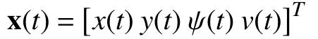

wheretrefers to time, (x,y) are longitudinal and lateral positions of the rear-wheel axis midpoint with the magnitude of velocity denoted byv, ψ ∈[-π,π] is heading angle,


B. Trajectory Planning
The trajectory planning is formulated in the form of an optimal control problem as follows
Optimal Control Problem 1 (OPT1):Find an admissible and bounded control input u*(t) that causes the system (1) to follow an admissible trajectory x*(t) that minimizes the performance measure
wheretfis the fixed final time and zr(t)=[xr(t)yr(t)]Tis the twice differentiable geometric reference path that both are given by the path planner.
The error terms are defined as
whereq1,q2,q3,q4,r1andr2are positive weights. Taking the derivative ofandin (1) gives


TABLE I COMPARISON OF METHODS

Fig. 1. Rear-wheel car-like robot model.
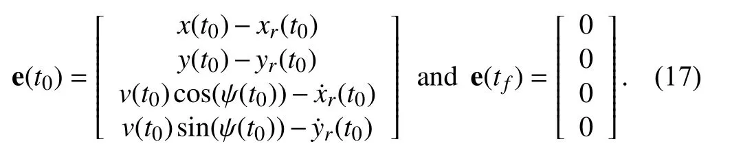
C. Boundary Conditions
The initial statesx(t0),y(t0), ψ (t0), andv(t0) follow the initial configuration of the vehicle, and they are not necessarily aligned with the reference trajectory, but considering the fact that the erroris expected to be zero at final timetf,

Accordingly, ψ (tf) andv(tf) can be found as

III. INPUT-OUTPUT LINEARIZATION TECHNIQUE
In order to simplify the problem formulation and circumvent dealing with the nonlinear differential equations,the input-output linearization technique is used as introduced in [4] to transform the nonlinear kinematic model (1) into a linear model from input to output. Since the system inputs explicitly appeared in the second derivative of the defined output z(t) in (5), it can be rewritten into the following matrix form

Definingan auxiliary input vector ζ (t)=[ζ1(t)ζ2(t)]Tgives

that results in two decoupled double integrators linearized from input to output as

The system has the relative degree 2 in the region


and define the error vector e(t) as

the tracking error state equationcan be written as follows

that is completely controllable. The OPT1 is reformulated as
Optimal Control Problem 2 (OPT2):Find an admissible control η*(t) that causes the system (14) to follow an admissible trajectory e*(t) that minimizes the performance measure

where

are positive definite weighted matrices.
Clearly, the boundary conditions are changed to
Remark 1:It should be noted that OPT2 is not a linear quadratic regulator (LQR) problem since, unlike the LQR problem formulation, e (tf) is assumed to be fixed.
IV. ANALYTICAL SOLUTION METHOD
Since the problem is minimizing the cost functional (15)subject to the tracking error state equations (14), the variational method is employed to solve the optimization. The proposed solution in this section is not only optimal but also guarantees the exponential stability of trajectory and control inputs.
A. Variational Method
Lemma 1:An optimal control η*(t) fort∈[t0,tf] which gives the optimal state e*(t) that minimizes the cost function(15) is the solution of the following two-point boundary value(TPBV) state linear differential equations

and co-state linear differential equations

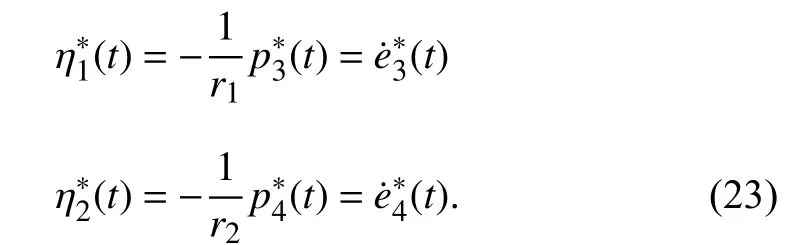
with boundary conditions in (17). The optimal control laws are also given by
Proof:To start solving the minimization (15), we form the Hamiltonian as follows

where the vector p(t)=[p1(t)p2(t)p3(t)p4(t)]Tincludes the Lagrange multipliers.
The necessary conditions of optimality are [17]
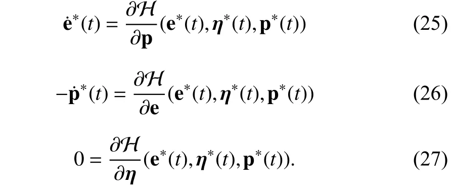
State and co-state equations are derived from the substitution of H(·) in (25) and (26), respectively. Also, (27)gives

from which the optimal control laws in (23) are obtained. ■
Taking the second and third derivative ofandfrom (19) and (20) gives
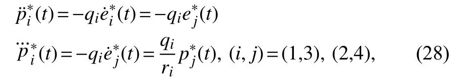
whereis given from substitution of (23) in (18). Similarly, substitutinginto the forth derivative ofgives

From (28), we have

which is a homogeneous linear ordinary differential equation.To solve the linear differential (30), the Laplace transform ofis first obtained as

wher e. From (28),is found as

Transforming (32) into the Laplace domain gives

Substitution of (31) in (33) gives


Taking the inverse Laplace transform of (31) and substituting the resultedinto the state and co-state equations gives the analytical optimal solution of the OPT2 problem with eight unknown parameters of, andwhich can be found to satisfy the eight initial and final boundary conditions in (17). However, (34) shows that the resultedis unbounded due to the right-half plane roots of the polynomialAlthough, this analytical solution can address the OPT2 assumptions, it fails to guarantee the stability of the system.
We approach the instability issue by relaxing e (tf) to be free while setting four of the initial conditions in (31) to cancel the unstable poles. The new assumption automatically changes the original problem to the infinite-time LQR problem formulated as follows.
Optimal Control Problem 3 (OPT3):Find an admissible control η*(t) that causes the origin e*=0 of the closed loop system (14) to be globally exponentially stable with an admissible trajectory e*(t) that minimizes the performance measure

where

are positive definite diagonal weighted matrices satisfying the boundary conditions

Underdampedfi>0:

Critically dampedfi=0:

Overdampedfi<0:

astfapproaches infinity.
B. Globally Exponentially Stable Analytical Solution
Theorem 1:The globally exponentially stable analytical solutions of the OPT3 are given by (38)-(46), where

andaiandbiare given as in Table II, which satisfy the initial boundary condition e (t0) in (17).


TABLE II ai AND bi FOR THREE DIFFERENT CASES

which gives

whereaiandbishould be determined by the initial boundary conditions. Sinceis a strictly-proper rational function ofs,is a time-invariant function [18]. Location of poles in(49) leads in three underdamped, critically damped, and overdamped solution cases:
1) Underdampedfi>0 : Ifhas complex roots, the inverse Laplace transform of (49) givesfort∈[t0,tf] as

By substituting the first derivative ofin (19) and (20),

2) Critically Dampedfi=0: This case occurs when the weights follow the equalityIn this case, the inverse Laplace transform of (49) givesfort∈[t0,tf] as

Substitution of its first and second derivatives in (19), (20),and (28) gives the closed form solution forandas in(41) and (42).
3) Overdampedfi<0: Equation (49) can be rewritten as
where |fi| is the absolute value offi. By taking the inverse Laplace of

Simil arly as the former cases,andare found as in(44) and (45). ■
Finding the errors give us the optimal states as

where
The optimal control inputs are found from (10) as

Remark 2:Sinceandare stable and a rctan(·) is the continuous function of its argument init can be concluded from (55) that the internal dynamics ψ*(t) andv*(t)are bounded.
C. Boundary Conditions Satisfaction
The parametersaiandbishould be set to satisfy the boundary conditions. Substituting the initial conditions (37)intoandgivesaiandbias illustrated for each case in Table II. As mentioned in Section IV-A, the final time boundary conditions may not be fulfilled since two unstable poles are eliminated in (31) to guarantee the stability, and the unknown parametersaiandbiare used up to satisfy the initial boundary conditions. However, the solution is a good approximation to satisfy e*(tf)≈0 due to the termse-c1i(tf-t0)ande-c2i(tf-t0)in overdamped, ande-mi(tf-t0)in underdamped and critically-damped cases. Thus, there exists a trade off between guaranteeing the stability, as proved for the OPT3 problem, and meeting the exact final time conditions as elaborated in the solutions of OPT2.
Remark 3:From (47) it can be concluded that for the fixed value ofri, if the values ofqi, andqjincrease by the factors ofand βi(for βi>1) , respectively, the values ofmifor the underdamped and critically damped cases,c1iandc2ifor the overdamped case will be increased as

which determines how fast the tracking errors converge to zero.
V. SIMULATION RESULTS
In this section, the effect of the weight change in controller performance, and tracking error is evaluated. At the end, the proposed closed-form solution in this paper is compared with other well-known methods in the literature. The simulations are developed in MATLAB. The reference time-parametrized trajectory, fort∈[0,30], is an eight-shaped Lissajous curve expressed as

The system starts from the initial configurations,x(0)=1.1,y(0)=0.8,v(0)=1, and ψ(0)=1.3, and the errors are expected to be zero at final time.
The tracking errors for three different cases are shown in Fig. 2. The errors can remain in a certain bound by making a trade-off amongqi,qj, andriweights. The impact of weight choice on the final time error can also be seen by decreasing the control effort that will increase the tracking time and consequently, it may unfavorably cause the final time error not to be close to zero. However, the trajectory error is globally exponentially stable and control inputs are guaranteed to be int∈[0,30].

Fig. 2. Tracking errors compared for different weighting parameters (UD =Underdamped, OD = Overdamped, and CD = Critically damped).
The vehicle trajectory, velocity, heading angle, and control variables, for three different cases, are illustrated in Figs. 3-5,respectively. As shown in Table III, the measured error e(tf)is almost zero attf= 30 s, 40 s, and 50 s for the three simulated cases, and converges to the zero for large enoughtfdue to the exponential stability of the solution. Boundedness of the control effort and internal dynamicsv*(t) and ψ*(t) are also evident in these figures.

Fig. 3. Weighting parameters impact on final time errors for the eightshaped trajectory tracking.
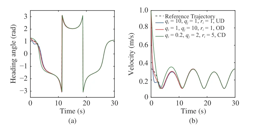
Fig. 4. Eight-shaped trajectory tracking: (a) heading angle: ψ *(t) and ψ r(t);(b) velocity: v *(t) and v r(t).

Fig. 5. Eight-shaped trajectory tracking: (a) steering angle: δ *(t); (b) acceleration: a *(t).
Finally, the proposed analytical solution in this paper is compared with our previous numerical solution (based on MATLAB two-point boundary value problem solution package BVP4C) in [19]. The integrand of cost function (3),i.e.,ep(·)2+ev(·)2+ea(·)2, is plotted over time in Fig. 6. The weights are set to beqi=1,qj=1, andri=1 for both cases.The cost function valueJ(·) for the analytical solution is9.87 which shows more than 380% reduction compared to the numerical case which gives 4 7.45.
VI. CONCLUSIONS AND FUTURE WORK
In this work, a novel globally exponentially stable trajectory optimization and tracking control formulation is proposed to generate the optimal trajectory and tracking control inputs for the car-like robot kinematic model.
The velocity and acceleration errors are minimized in addition to the position error, which allows us to extract the optimal control u*(t) without considering any parametrized geometric function representations for control inputs since they explicitly appear in the cost function. The input-outputlinearization technique is employed to linearize the system from the defined auxiliary input to output. The closed-form optimal trajectories and control inputs are obtained by the calculus of variation technique, and boundedness of the solution and internal dynamics are also proved.

TABLE III ERROR MEASUREMENTS AT THREE TIME INSTANCES(t f =30 s , t f =40 s, AND t f =50 s).

Fig. 6. Comparison of analytical and numerical methods based on their measured cost function integrand, i.e., e p(·)2+ev(·)2+ea(·)2, over time.
The proposed framework can be easily extended to tackle the optimal trajectory optimization problem of a higher dimensional kinematic model with more states by adding the higher order derivatives of thex(t) andy(t) into the cost function and assuming that the reference trajectory is smooth.
Our proposed optimal planning framework is an open loop control strategy which yields continuous control signals(sequence of inputs) as a function of the initial state of the vehicle. Thus, if the states evolves exactly according to the model then the predicted state trajectory is exactly obtained in reality by applying the calculated optimal input signal.However, if the model is inaccurate and the system is subject to disturbance not included in the model, the result of applying the open-loop control signal may be different than what is expected. Thus, in our future work, we aim to apply the repeated application of this open-loop strategy in discretetime domain to obtain the same feedback effect of recursive techniques, known as receding horizon strategy in the literature.
 IEEE/CAA Journal of Automatica Sinica2020年1期
- IEEE/CAA Journal of Automatica Sinica的其它文章
- Networked Control Systems:A Survey of Trends and Techniques
- Big Data Analytics in Telecommunications: Literature Review and Architecture Recommendations
- A New Robust Adaptive Neural Network Backstepping Control for Single Machine Infinite Power System With TCSC
- Algorithms to Compute the Largest Invariant Set Contained in an Algebraic Set for Continuous-Time and Discrete-Time Nonlinear Systems
- Asynchronous Observer Design for Switched Linear Systems: A Tube-Based Approach
- Deep Imitation Learning for Autonomous Vehicles Based on Convolutional Neural Networks