Algorithms to Compute the Largest Invariant Set Contained in an Algebraic Set for Continuous-Time and Discrete-Time Nonlinear Systems

Laura Menini, Corrado Possieri, and Antonio Tornambè

Abstract—In this paper, some computational tools are proposed to determine the largest invariant set, with respect to either a continuous-time or a discrete-time system, that is contained in an algebraic set. In particular, it is shown that if the vector field governing the dynamics of the system is polynomial and the considered analytic set is a variety, then algorithms from algebraic geometry can be used to solve the considered problem. Examples of applications of the method (spanning from the characterization of the stability to the computation of the zero dynamics) are given all throughout the paper.

I. INTRODUCTION

THE “second method” of Lyapunov, which makes use of a function that is monotonically decreasing along the solution of a system, is one of the most widespread and literature pervasive tools to characterize the stability of nonlinear system [1]-[9], such a method has been generalized in order to possibly deal with monotonically non-increasing functions, by exploiting the concept of invariant set. Since these seminal works, the notion of invariant set has been extensively used in order to characterize the properties of nonlinear dynamical systems. For example, in [10], invariant sets are used to characterize the disturbances that let the output of a discrete-time,linear system vanish identically, in [11], controlled invariant sets are used to solve the disturbance decoupling problem, in[12], invariant sets are used to characterize some observability properties, and, in [13], (controlled) invariant sets are used to extend the notion of zero to nonlinear dynamical systems(see also [14] for a comprehensive review of the literature about the output zeroing problem and the zero dynamics of a system).

Due to the importance of invariant sets in both theoretical research and engineering practice (especially when dealing with stability of nonlinear dynamical system), a lot of research effort has been carried out to characterize such sets [4], [15],[16]-[20].

The main objective of this paper is to provide computational tools to determine the largest invariant set, with respect to either a continuous-time or a discrete-time nonlinear system,that is contained in an algebraic set. Such a problem is crucial in several control applications, as shown by the subsequent Theorems 1 and 6, that require the solution to such a problem to guarantee asymptotic stability of a given set. The goal of computing such an invariant set is pursued by showing that this set can be determined by solving a set of analytic equations. Furthermore, it is shown that, if the vector field governing the dynamics of the system is polynomial and the algebraic set is an affine variety, the largest invariant set with respect to the system that is contained in the affine variety can be determined through computationally efficient algorithms,which use tools borrowed from algebraic geometry that have already been used to solve control problems, such as observer design [21], [22], generation of algebraic certificates of(possibly, asymptotic) stability [23], solving the equations that arise in the harmonic balancing method [24], multi-objective optimal design of controllers for linear plants [25], checking the controllability of polynomial systems [26], and motion planning of mobile robots [27], [28]. Examples are given all throughout the paper to illustrate and corroborate the theoretical results. Applications of the proposed methods to several control problems are reported as, e.g., stability analysis of nonlinear systems, test of the zero-state observability property, solution to the output zeroing problem,computation of the zero dynamics of a nonlinear plant.

The results given in this paper are related to the ones concerning the output zeroing of nonlinear autonomous systems [29]-[31]. The main difference between the results given in this paper and the ones available in the literature is that herein algorithmic procedures (ready to be implemented in CAS software, such as Macaulay2 [32]) are proposed to determine the largest invariant set that is contained in an algebraic set with respect to either a continuous-time or a discrete-time analytic (possibly, polynomial) system.

Organization of the paper: the notation used in this paper is introduced in Section II, together with some preliminary results. The problem of determining the largest invariant set,which is contained in an analytic set, with respect to either a continuous-time or a discrete-time system is addressed in Sections III and IV, respectively. Examples of application of the given methods are reported in Section V. Conclusions are given in Section VI.

II. NOTATION AND PRELIMINARIES

Given a multi-index

is the variety generated byp1,...,pℓ. Similarly, given an idealinthe variety of the ideal I is the set

A monomial order ≻ is a total well ordering relation among the monomialsOnce a monomial order ≻ is fixed(such as the LEX order defined in [33]), any polynomialcan be rewritten aswherei=1,...,m, andThus,the leading term and the leading coefficient ofpareand LC(p)=c1, respectively. Once a monomial order ≻ is fixed, the setwith 〈g1,...,gs〉=I,is a Gröbner basis of an ideal I in R [x] if

A functionis smooth in its domain of definition(assumed to be open) ifqis C∞at eachIf, a power series can be associated with the smooth functionqlocally aboutx0as follows:

A smooth functionqis locally analytic inx0if there exists an open neighborhoodofx0such that the series in (2)converges andq(x)=Q(x), for eachx∈B;qis analytic inif it is locally analytic in each

Givenand smooth functionsanddefine theith directional derivative ofhalongfasandand theith directional successor ofhalongfasand

Given analytic functionsdefine the analytic set

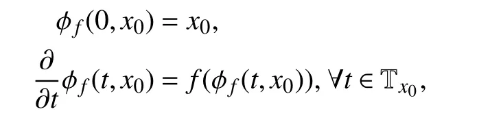
wherex=[x1...xn]T, and the vector fieldis analytic inwithbeing an open subset of. Assume,without loss of generality, that the initial time is 0. The response at timetof system (3) from the initial stateis denotedis theCT-flowassociated withfand satisfies (see [34])

Definition 1:A setis positively (respectively,negatively)f-invariant if, for eachx0∈S , φf(t,x0)∈S,(respectively,A set S isf-invariant if it is both positively and negativelyf-invariant.

Hence, consider the following problem.

Problem 1:Let functionsanalytic inbe given. Find the largestf-invariant set contained in

The availability of tools to determine a solution to Problem 1 is crucial in several control applications and, in particular,for the application of the next two theorems.

Theorem 1 (Lyapunov stability [4]):Let 0 be an equilibrium of system (3) and assume thatLetV:be a differentiable, radially unbounded, positive definite function such thatLf V(x)≤0, ∀x∈Rn. If the largestf-invariant set inis {0} , then 0 is globally asymptotically stable.

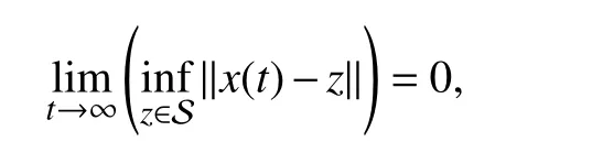
Theorem 2 (Invariance principle [35]):Letbe a compact, positivelyf-invariant set. Letbe analytic in Ω and such thatLf V(x)≤0, ∀x∈Ω. Let S ⊂Ω be the largestf-invariant set in. Every responsex(t) of system (3) starting in Ω approaches S , i.e.,

III. INVARIANT SETS FOR CONTINUOUS-TIME SYSTEMS Consider the continuous-time, time-invariant system

In order to apply Theorem 1, one has to guarantee that S={0} is the solution to Problem 1 withh=Lf V(x). On the other hand, in order to apply Theorem 2 to prove attractiveness of the set S, one has to guarantee that S is the largest invariant set that is contained in, i.e., that S is the solution to Problem 1 withh=Lf V(x), and that the set Ωis positively invariant. It is worth noticing that if, in addition to the hypotheses of Theorem 2, the functionVis positive definite and there isc＞0, such thatis a subset ofand is compact, then, by classical Lyapunov results [4], the setis positively invariant (and contractive).

Remark 1:The LaSalle invariance principle recalled in Theorem 2 has already been used in [36], [37] to determine estimates of the region of attraction of an equilibrium point via polynomial optimization techniques, such as sum of squares tools. The main difference between such techniques and the ones given in this paper is that the former allow one to determine positivelyf-invariant sets that constitute inner estimates of the region of attraction of an asymptotically stable equilibrium point, whereas the latter allow to determine algebraically the largestf-invariant set S contained in a variety (such as, e.g.,i.e., under the hypotheses of Theorem 2, they allow one to characterize the set to which the trajectories of system (3) converge rather than its region of attraction.

In the following Section III-A, a method to determine the solution to Problem 1 in the analytic case is proposed. An algorithm, which uses the algebraic geometry tools recalled in Section II, is given in Section III-B to apply such a technique in the polynomial case.

A. Solution to Problem 1 in the Analytic Case

The main objective of this subsection is to provide a solution to Problem 1 whenfandh1,...,hmare analytic functions, but not necessarily polynomial. To this end,consider the following remark.

Remark 2:Letbe analytic in some intervalpossibly coincident with R. Letbe any open subinterval ofOne has that α(t) is equal tocfor allfor some constantif and only if α(t) is equal tocfor allTherefore, for anyt0in the interior of, α(t) is equal tocfor allif and only if α(t0)=candk＞0.

Following Remark 2, the next lemma provides necessary and sufficient conditions ensuring that a functionhvanishes identically along the CT-flow φf(t,x0).

Lemma 1:Letf:andbe analytic inFor eachone hash(φf(t,x0))=0 ,if and only if∀i∈Z≥0.

Proof:Sincefandhare analytic infor any, one has thath(φf(t,x0)) is an analytic function oftinHence,sincefor alltif and only ifh(φf(t,x0))=0 for allwhereis a sufficiently small neighborhood of 0. Since

one has thath(φf(t,x0)) vanishes identically if and only if

The results given in Lemma 1 are used in the following lemma to prove that the largest positively (respectively,negatively)f-invariant subset ofis the largestfinvariant subset of

Lemma 2:Ifis the largest positively (respectively,negatively)f-invariant set contained in, then it is the largestf-invariant set contained in

Proof:Letx0∈S be fixed. Thus, letbe the maximal interval of existence of φf(t,x0) . Since S is the largest positivelyf-invariant set contained inthere existssuch thatqj(φf(t,x0))=0 for allt∈[0,T],j=1,2,.... By Lemma 1, if there exists a responsex(t) of system (3) such thatqj(x(t))=0, ∀t∈[0,T], for somethenTherefore, sincex0can be chosen arbitrarily in S and there does not existsuch that, for alland(otherwisewould be in S) , S is the largestf-invariant set contained in

By using Lemma 2, the following theorem shows how to determine the solution to Problem 1 in the analytic case.

Theorem 3:Letandbe analytic functions in U. The largestf-invariant set contained inis

The following example shows how Theorem 3 can be used to determine the solution to Problem 1.

Example 1:Consider the following system

whereqi(x) is a globally analytic function for each(namely,q0(x)=1,q1(x)=cos(x1),q2=sin2(x2)+cos(x1)×cos(x2), and so on). Therefore, sincethe largest invariant w.r.t. system (4) contained inis

In order to apply Theorem 3, one has to compute the intersection of infinitely many sets, i.e.

Proof:By Lemma 2, the largestf-invariant set contained inis

By Lemma 1,hj(φf(t,x))=0 for allif and only if

and leth(x)=sin(x1). It can be easily derived that

Hence, consider the following proposition, which show how these computations can be simplified.

Proposition 1:Assume that there exist a set {q1,...,qℓ} of analytic functions insuch that

Fig. 1. Phase plot of system (4) (blue), algebraic set (green), and invariant set S (red).

for some αk,χ,k=1,...,ℓ , being analytic in. Hence, there exist functionsbeing analytic insuch that=1,...,ℓ ,i∈Z≥0. Furthermore, ifthenqi(φf(t,x0))=0,i=1,...,ℓ, for allt∈Tx0.

Proof:The proof is carried out by induction. By assumption, there exist analytic functions αj,ksuch that

Thus, the statement holds fori=1. Assume now that, fori∈Z≥0, there exist analytic functions βi,j,ksuch that. Therefore,

which is a linear combination ofq1,...,qℓ, with analytic coefficients in U. Thus, ifqj(x0)=0 for allj=1,...,ℓ, thenfor allHence, the proof follows by Lemma 1. ■

By Proposition 1, if there existssuch that each

Therefore, if such an assumption holds, then the computations to be carried out so to find a solution to Problem 1 involve just a finite number of intersections, as shown in the next example.

Example 2:Consider the following system (p. 214 of [38]):

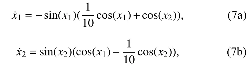
Therefore, since there exists an analytic function α such thatLf h(x)=α(x)h(x), by Proposition 1, the largestf-invariant set contained inFig. 2 depicts the phase plot of system (7) and

Fig. 2. Phase plot of system (7) (blue curves), algebraic set (green),and f-invariant set S (red).

Example 3:Consider the system given in Ex. 8, Ch. 9 of[38]

it is immediate to see that it cannot be expressed as α(x)h(x),for some α(x) analytic on the whole R2. Similarly, it is not trivial to determine whether

can be expressed as a linear combination ofhandLf h.However, algebraic geometry can be used to solve this problem, as suggested in Chapter 6 of [33]. Introduce the auxiliary single variablesc1,c2,s1,s2, and fix inthe LEX order ≻, withConsider the polynomial -c1c2obtained by replacing cos(x1) and cos(x2) inLf h(x) withc1andc2, respectively; consider the ideal J1generated byx2,c1c2and by thei=1,2, where the polynomialarises from the equality sin2(xi)+cos2(xi)=1, with similar substitutions. In the same way, consider the polynomialwhich arises fromBy computingp2%J1=c2s2≠0, one obtains thatp2cannot be expressed as a polynomial sum of the generators ofwhencecannot be expressed as a linear combination ofhandLf h. Thus, computeand its associated polynomialHence, by letting

one obtains thatwhencecan be expressed as a linear combination ofThus, by Proposition 1,the solution to Problem 1 is given by

Fig. 3 shows the phase plot of system (8),and S.

Fig. 3. Phase plot of system (8) (blue), algebraic set (green), and invariant set S (red).

Note that, although for many analytic systems there isN∈Z≥0such thatcan be expressed as a linear combination of...,m,i=0,...,N, this need not always hold, as shown in the following counterexample,which shows that the solution to Problem 1 need not be computable as a finite intersection, as in (6).

Example 4:Consider the system

By [41], the functionh:R →R is analytic in R,andfori=1,2,..., andj=1,2,3,.... Since it results thatandh(N+1)=0,...,=0,there is nosuch thatcan be expressed as a linear combination of. Namely, for each

whereas the largestf-invariant set contained inis

i.e., the set S cannot be determined with a finite number of intersections.

In the following subsection, it is shown that, if bothfandhare polynomial functions, then there always existsN∈Z≥0such thatcan be expressed as a weighted sum ofwith polynomial weights, thus allowing the design of an algorithm to solve Problem 1.

B. Solution to Problem 1 in the Polynomial Case

The main objective of this subsection is to show that the computations required to determine the solution to Problem 1 are much simpler when the entries offandh1,...,hmare inwhich implies that

Consider the following lemma.

Lemma 3:Let a countable (possibly, infinite) sequence of polynomialsp1,p2,... inbe given. There exists a finite number of polynomialssuch that:

Proof:LetandSinceis an ascending chain of ideals inby Theorem 7 at p. 80 of [33], there isN≥1 such thatBy Theorem 4 at p. 190 of[33],

Lemma 3 suggests that, in order to determine a solution to Problem 1 by using the expression given in (5), if both the entries offandh1,...,hmare polynomials, then S can be obtained by computing the intersection of a finite number of varieties. In the remainder of this subsection, it is shown how such computations can be carried out by using the algebraic geometry tools recalled in Section II.

Let a monomial order ≻ be fixed. Given an ideal I in R[x],letbe the reduced Gröbner basis of I with respect to ≻. The directional derivativeLfI of I alongfis the ideal defined as follows:

Given a polynomialpin some ideal I, the next lemma states that the directional derivative alongfofpbelongs to the sum of I and of its directional derivativeLfI.

Lemma 4:Iff∈Rn[x] and I is an ideal in R[x], thenp∈I implies that

Proof:Ifp∈I, then, letting 〈p1,...,pℓ〉=:I, there exist α1,...,αℓ∈R[x] such thatThus, one has

The following statement extends the results of Lemma 4 to theith directional derivative of a polynomial.

Lemma 5:Iff∈Rn[x] and I is an ideal in R[x], define the sequence of ideals I0,I1,I2,... iteratively as

p∈I

Hence, if,then

Proof:The lemma is proved by induction. The base of the induction is proved by Lemma 4 by lettingi=1. As for the inductive step, assume that for somei∈Z≥0, ifp∈I0, thenSinceand Ii+1=Ii+LfIi, by Lemma 4, one has that

Consider the ideals I0,I1,I2,... defined as in (10). The following lemma states that there is an element INof such a sequence such thatfor allj∈Z≥0.

Lemma 6:Iff∈Rn[x] and I is an ideal in R[x], define I0,I1,I2,... as in (10). Hence, there isN∈Z≥0, such thatfor alli∈Z≥0and allj∈{1,...,m}.

Proof:Since I0⊂I1⊂I2⊂... is an ascending chain of ideals in R[x], by Theorem 7 at p. 80 of [33], there existsN∈Z≥0such that IN+j=INfor allj∈Z≥0. By Lemma 5,, for alli∈Z≥0.

By combining the results given in Theorem 3 and Lemmas 3 and 6, the following lemma shows that if I0=〈h1,...,hm〉,thenis the solution to Problem 1.

Lemma 7:Let I =〈h1,...,hm〉 and define I0,I1,I2... as in Lemma 6. Hence, the solution to Problem 1 is V (IN).

The following example shows how to use the results given in Lemma 7 to determine the solution to Problem 1.

Example 5:The objective of this example is to study the stability of the origin of

Consider the candidate Lyapunov function

Thus, the largestf-invariant set contained in V(Lf V(x)) isand, by Theorem 1, the origin is globally asymptotically stable.

As shown by Example 5, in order to apply the method proposed in Lemma 7 to solve Problem 1, one has to compute a large number of reduced Gröbner bases. In the following, it will be shown that such computations can be reduced by exploiting the concept of the radical of an ideal. In fact, letting I0,I1,I2,... be defined as in (10), letBy Lemma 6, there issuch thatj∈Z≥0. Thus, consider the next lemma, whose proof follows by Lem. 5 at p. 182 of [33].

Lemma 8:Assume thatf∈Rn[x] andh1,...,hm∈R[x]. Let I=〈h1,...,hm〉, define I0,I1,I2,... as in (10), and letThere issuch thatfor alli∈Z≥0andj∈{1,...,m}.

The following lemma shows how to determine an idealcontainingfori∈Z≥0andj∈{1,...,m}.

Lemma 9:Assume thatandThus,define the sequence of idealsas

Proof:By induction, it is proved thatfor alli∈Z≥0and allj∈{1,...,m}. Leti=0. Clearly,hj∈〈h1,...,hm〉, whence by Lemma 5 at p. 182 of [33],Now, for anyi∈Z≥0, assume thatBy Lemma 4, since one has thatwhence

by Lemma 5 at p. 182 of [33]. Sinceis an ascending chain of ideals inby Theorem 7 at p. 80 of[33], there existssuch thatfor allj∈Z≥0.

In the following theorem, whose proof follows directly from Theorem 3 and Lemma 9, a method is proposed to determine a solution to Problem 1 in the polynomial case.

Theorem 4:Assume thatf∈Rn[x] andh1,...,hm∈R[x],and defineas in (11). Lettingbe such thatfor allthe largestf-invariant set contained inis

The following Algorithm 1 summarizes the computations that have to be carried out to solve Problem 1 in the polynomial case by using Theorem 4.

Algorithm 1 Solution to Problem 1

Note that in order to apply Algorithm 1, just the knowledge of the polynomialfandh1,...,hmis required. Once a monomial order is fixed, Step 2 of Algorithm 1 can be carried out by comparing the reduced Gröbner basesandof the respective idealsandAs a matter of fact, by Theorem 5 at p. 120 of [33], for a given monomial order, each ideal has a unique reduced Gröbner basis, whenceif and only ifNote that, by Lemma 9, such an algorithm entails a finite number of iterations. The following Fig. 4 illustrates Algorithm 1.

Fig. 4. Illustration of Algorithm 1.

The following example is an application of Algorithm 1.

Example 6:Consider again the system and the Lyapunov functionVgiven in Example 5. By using Algorithm 1 with inputfandLf V, one obtains thatandThus, sincethe algorithm terminates by returningNote that, in order to obtain the same result by using Lemma 6, one has to compute the reduced Gröbner bases of 9 ideals, whereas, by using Algorithm 1, just 3 reduced Gröbner bases have to be computed.

The following remark details how to compute the restriction of the dynamics (3) to anf-invariant set S .

Remark 3:By [42], if the set S isf-invariant andis not a critical point, thenfis tangent to S inthus allowing to easily determine the restriction of the dynamics of system(3) to the set S. As a matter of fact, define

and the tangent space of S inas

By [33], if S=〈p1,...,pℓ〉, thenwhich is a translation of a linear subspace of Rn, i.e., there existb1,...,bs∈Rn(dependent onsuch thatTherefore, for each non-criticalone hasi.e., there existc1,...,cs∈R

(dependent onsuch that

This parametrization constitutes the restriction of the dynamics (3) to S.

IV. INVARIANT SETS FOR DISCRETE-TIME SYSTEMS Consider the discrete-time, time-invariant system

Definition 2:The setis

● positivelyf-invariantiff(S)⊂S;

● negativelyf-invariantiff(S)⊃S;

●f-invariantiff(S)=S.

The main goal of this section, formalized in the following problem, is to determine the largest positivelyf-invariant set contained in an analytic set.

Problem 2:Let functionsbe analytic in U. Find the largest positivelyf-invariant set contained in V (h1,...,hm).

Note that, for discrete-time systems, the attention can be focused just on positivelyf-invariant sets, when considering the following two theorems.

Theorem 5 (Invariance principle [5], [43]):Let Ω be a subset of U and letV:Ω →R be a continuous function such that Δf V(x)-V(x)≤0 for allx∈Ω. Let S be the largest positivelyf-invariant set contained inwhereis the closure of Ω . If ψf(t,x0)∈Ω for allt∈Z≥0and ψf(t,x0) is bounded, then there existssuch thatast→∞.

Theorem 6 (Lyapunov stability [44]):Letand letbe differentiable, radially unbounded, and positive definite. If Δf V(x)-V(x)≤0 for allx∈Rn, then any response of system (12) tends to the largest positivelyf-invariant set contained in

Note that, in order to apply both Theorems 5 and 6, one has to determine the largest positivelyf-invariant set contained inf

In the following Section IV-A, a method to determine the solution to Problem 2 in the analytic case is proposed. An algorithm, which uses the algebraic geometry tools recalled in Section II, is given in Section IV-B to apply such a technique in the polynomial case.

A. Solution to Problem 2 in the Analytic Case

The main objective of this section is to provide a solution to Problem 2 when both the entries offandh1,...,hmare analytic in U. Consider the following lemma.

Lemma 10 (Existence of responses [45]):The DT-flow ψf(t,x0) is well defined for each

Note that the statement of Lemma 10 holds just fort∈Z≥0.On the other hand, uniqueness of the responses of system (12)need not hold backward in time, sincefneed not be bijective.Consider the following theorem, which shows how to determine the solution to Problem 2 in the analytic case.

Theorem 7:Letandj=1,...,m, be analytic functions in U. The largestf-invariant set contained inis

Proof:By the definition of the DT-flow ψf(·,·) and by Lemma 10, for allandone has that

Therefore, since the largest positivelyf-invariant set contained in V (h1,...,hs) is

this set equals the set given in (13).

In order to apply the technique proposed in Theorem 7 to solve Problem 2, one has to compute the intersection of infinitely many sets, i.e.,

As for continuous-time systems, such computations can be simplified, as shown in the following proposition, whose proof is similar to the proof of Proposition 1.

Proposition 2:Assume that there exist a set {q1,...,qℓ} of analytic functions in U such that

for some αk,χ,k=1,...,ℓ , being analytic in U. Hence, there exist βi,j,kbeing analytic in U such that, forj=1,...,ℓ,

Moreover, ifq1(x0)=···=qℓ(x0)=0 thenq1(x(k))=···=qℓ(x(k)), for allk∈Z≥0.

By Proposition 2, if there isN∈Z≥0such thatcan be expressed as a linear combination of,...,m,i=0,...,N, with analytic coefficients, then

i.e., as for continuous-time systems, just the intersection of a finite number of sets needs to be determined.

Example 7:Consider the system [43]

By Theorem 6, trajectories of (16) tend to S. Fig. 5 depicts some trajectories of system (16).

Fig. 5. Set V (h) (green), positively invariant set S (red), and trajectories of system (16).

In the following subsection, it is shown that, if bothfandhare polynomial functions, then there existsN∈Z≥0such thatcan be expressed as a linear combination ofthus allowing the design of an algorithm to solve Problem 2.

B. Solution to Problem 2 in the Polynomial Case

The main objective of this subsection is to show that the computations required to solve Problem 2 are simpler in case of polynomial systems, for which U=Rn. By Lemma 3, iff∈Rn[x] andh1,...,hm∈R[x], then the set S given in (14)can be determined by computing a finite number of intersections. In the following, it is shown how such computations can be carried out by using the tools recalled in Section II.

Let a monomial order ≻ be fixed. Given an ideal I in R [x],letbe the reduced Gröbner basis of I. The directional successor of I alongfis

Given a polynomialpin some ideal I, the next lemma states that the directional increment alongfofpbelongs to the sum of I and of its directional increment ΔfI.

f∈Rn[x] I R[x]p∈I

Lemma 11:If and is an ideal in , then implies that

In view of Lemma 11, consider the following lemma.

Lemma 12:Iff∈Rn[x] andh1,...,hm∈R[x], then define the sequence of ideals I0,I1,I2,... as

There existsN∈Z≥0such that

Furthermore, the solution to Problem 2 is V (IN).

Proof:Note that the sequence I0,I1,... is such that

The following example shows how the tool given in Lemma 12 can be used to solve Problem 2.

Example 8:Consider the following system

Consider the candidate Lyapunov functionIt can be easily seen that

which is negative semi-definite about the origin. Now, one can compute the largest positivelyf-invariant set contained in V(Δf V(x)-V(x))by using the sequence of ideals defined in Lemma 12. Thus, letI1=I0+ΔfI0and I2=I1+ΔfI1. By computing the reduced Gröbner basesandof I1and I2, respectively, one haswhence I1=I2. In particular, the reduced Gröbner basis of I1iswhere:

Thus, by Lemma 12, the largest positivelyf-invariant set contained inis

As for continuous-time systems, the concept of radical of an ideal can be used to reduce the number of Gröbner bases to be computed, as shown in the following theorem.

Theorem 8:Assume thatf∈Rn[x] andh∈Rm[x]. Define the sequence of ideals K0,K1,K2,... as

There existssuch thatj∈{1,...,m} , and such that the largest positivelyf-invariant set contained in

Proof:First, it is proved, by induction, that

Since, by Lemma 5 at p. 182 of [33],one has that (21) holds fori=0. Assume now that (21) holds for someHence, by Lemma 11,

thus concluding the induction.

Secondly, it is proved that there existssuch thatfor allj∈Z≥0. By considering that

is an ascending chain of ideals in R [x], by Theorem 7 at p. 80 of [33], there existssuch thatfor allj∈Z≥0. The proof is concluded by the fact that, by Theorem 7, the largest positivelyf-invariant set contained in V(h1,...,hm) is given by V (h1,...,hm,Δf h1,...).

The following Algorithm 2 resumes the computations to be carried out to solve Problem 2 in the polynomial case by using the method outlined in Theorem 8.

Note that, as for Algorithm 1, in order to apply Algorithm 2,just the knowledge of the polynomialfandh1,...,hmis required. The following Fig. 6 illustrates Algorithm 2.

Fig. 6. Illustration of Algorithm 2.

The following remark details how to determine the restriction of the dynamics (12) to S in a particular case.

Algorithm 2 Solution to Problem 2.

Remark 4:If the variety S is rational (i.e., there exists∈Z≥0and rational mappingssuch thatfor allx∈S andfor all σ ∈Rs), then the restriction of the dynamics (12) to S can be easily determined. Namely, lettings∈Z≥0be the dimension of S, the dynamics of system (12) restricted to S are

V. EXAMPLES OF APPLICATION OF THE GIVEN METHODS

In this section, several examples are given in order to illustrate the application of the proposed methods.

The following example shows how Algorithm 1 can be used to determine the set of initial conditions that make the output of a linear system be identically zero.

Example 9:Consider the linear system obtained either from(3) or from (12) by lettingf(x)=Ax, with

Consider the linear functionh(x)=Cx, where

(iv) if (a1-a2)c2=0,c1=0, one has three cases:

(iv.a) if, then S =V(x2);

a1≠a2c2=0 S=R2

(iv.b) if , , then ;

a1=a2c2=0 S=R2

(iv.c) if , , then .

The following example illustrates how the proposed methods can be used to study the stability of a mechanical system by using its energy as Lyapunov function.

Example 10:Consider the mechanical system depicted in Fig. 7, whose dynamics are given by, where

Fig. 7. A mechanical system.

x(t)∈R4represents the positions and velocities of the two bodies having massm,kis the stiffness of the springs anddis the damping coefficient of the damper.

Consider the candidate Lyapunov function

which is the total energy of the system. It can be easily derived thatLf V=-d(x2-x4)2≤0. Therefore, the origin of the considered system is stable (actually, the sub-level set{x∈R4:V(x)≤c} is positively invariant for anyc∈R≥0). By using Algorithm 1 with inputf(x)=Axandh(x)=Lf V(x),one obtainsand K2=K1. Thus, the largest invariant set contained in V(Lf V)is S=V(x2-x4,x1-x3). Thus, by Theorem 2, every solution ofxapproaches S ast→∞.

The methods given in this paper can be used even if in the largestf-invariant set contained in V(h1,...,hm) there is a limit cycle, as shown in the next example.

Example11:Consider system (3) withwhich has been obtained by using [27, Alg. 1] and imposingas limit cycle. Lettingnote thatthus implying that sub-level sets ofVare positively invariant. By using Algorithm 1 with inputf(x) andh(x)=Lf V(x), one obtainsandThus, the largestf-invariant set contained in V (Lf V) is

The following example shows how the given tools can be used to study the behavior of an averaging algorithm.

Example 12:Consider the equal-neighbor averaging model[46]x(t+1)=Ax(t), with

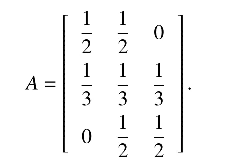
Consider the candidate Lyapunov function

By using the “complete the squares” procedure [23], one obtains that Δf V-Vcan be written as

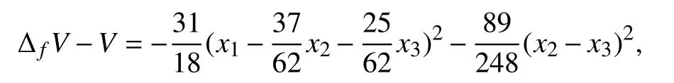
thus guaranteeing that the sub-level sets ofVare positively invariant. By using Algorithm 2 with inputf(x)=Axandh(x)=Δf V(x)-V(x), one obtains K0=〈h〉 andThus, the largest positively invariant set with respect tox(k+1)=Ax(k) contained in V(h)is S =V(x1-x2,x2-x3). Hence, by Theorem 5, each bounded solution of the considered averaging algorithm tends to S.

The following example shows how Algorithm 1 can be used, with minor modifications, to solve the output zeroing problem and to determine the zero dynamics of a nonlinear controlled system.

Example 13:Consider the system given in Example 6.1.6 of[42],=f(x)+g(x)u,y=η(x), where

andy(t)∈R2are the control and output vectors, respectively. The objective of this example is to determine the set of initial conditions and control inputs that make the output of the system be identically zero. By the same reasoning used to prove Lemma 1, one has thaty(t)=0 for all admissiblet∈R if and only if all of its time derivatives vanish. Thus, by computing the time derivative of the output up to the third order, one obtains a set of polynomials in the state of the system and the time derivatives of the input, up to the second order. By computing the reduced Gröbner basis of the corresponding ideal, one obtains

where

Thus, by lettingand lettingh(x)=[x1x2x4x5]T, and by using Algorithm 1 with inputandh, one obtains that the set S =V(h) is the largest invariant set with respect tocontained in V(h).Therefore, the control inputand the set S solve the output zeroing problem. Thus, the method given in Remark 3 can be used to determine the zero dynamics of the system. In fact,Tx¯(S)=V(x1,x2,x4,x5) for eachand the restriction off*(x) to S is

whence the zero dynamics of the system areNote that the same result has been obtained in [42], by using different arguments.

It is worth noticing that the procedure outlined in Example 13 does not require neither that the system is input affine nor that the number of inputs is equal to the number of outputs, as shown in the following example.

Example 14:Consider the plant

By computing the time derivatives of the output, the reduced Gröbner basis of the corresponding ideal is that the largest invariant set with respect to the system

Thus, by lettingandh(x)=η(x), one obtainscontained in V(h) is S=V(h). Therefore,and S solve the output zeroing problem. The method given in Remark 3 can be used to determine the zero dynamics of the system. In fact, one has thatfor eachand the restriction of the vector fieldf*(x) to S isThus, the zero dynamics of the system are

The following example shows how Algorithm 2 can be used to characterize the observability of system (12) from the output. Consider the discrete-time system

System (23) is zero-state observable ify(t)=0,t∈Z≥0,impliesx(t)=0,k∈Z≥0[44].

Example 15:Consider system (23), with

By using Algorithm 2 with inputfandh, one obtains thatandThus, the algorithm returns as outputi.e., the largest positivelyf-invariant set such thaty(t)=0 for allt∈Z≥0is {0}, whence the system is zero-state observable.

VI. CONCLUSIONS

In this paper, some computational tools have been proposed to determine the largest invariant set contained in an analytic set, in the case of both continuous-time and discrete-time nonlinear systems. In particular, it has been shown that, if the vector field governing the dynamics of the system is analytic,such a set can be computed by determining the set of all the solutions of a system of (possibly, infinite) analytic equalities.On the other hand, if the vector field is polynomial and the algebraic set is a variety, then this set can be determined with a finite number of steps. Several applications to control problems have been reported. In fact, as shown in Section V,the techniques proposed in this paper can be used to determine the set of initial conditions that make the output of a linear system be identically zero, to study the stability of dynamical systems, to characterize the behavior of averaging algorithms,to solve the output zeroing problem, to determine the zero dynamics of a nonlinear controlled system, and to characterize the zero-state observability of autonomous nonlinear systems.

Future developments of the techniques given in this paper will deal with the extension of the proposed algorithms to the hybrid case, i.e., to systems presenting both continuous-time and discrete-time dynamics.

Note that Algorithms 1 and 2 are computationally tractable in many cases of practical interest. In fact, although computing Gröbner bases is, in the worst case, an EXPSPACE-complete problem [48], in the generic case,Gröbner bases can be computed efficiently by the most recent algorithms and hence the algorithms given herein can be actually employed (see [49], [50] for further details).

Therefore, although the main limitation of the proposed approach is the computation of Gröbner bases of the idealsit may be used to solve problems of practical interest. For instance, an implementation of Algorithm 1 in Macaulay2 has been used to solve Problem 1 withfandhbeing polynomials in 10 variables of degree 6 within reasonable computing time.