Quantum partial least squares regression algorithm for multiple correlation problem

Yan-Yan Hou(侯艳艳) Jian Li(李剑) Xiu-Bo Chen(陈秀波) and Yuan Tian(田源)

1School of Artificial Intelligence,Beijing University of Post and Telecommunications,Beijing 100876,China

2College of Information Science and Engineering,Zaozhuang University,Zaozhuang 277160,China

3Information Security Center,State Key Laboratory of Networking and Switching Technology,Beijing University of Post and Telecommunications,Beijing 100876,China

4GuiZhou University,Guizhou Provincial Key Laboratory of Public Big Data,Guiyang 550025,China

Keywords: quantum machine learning,partial least squares regression,eigenvalue decomposition

1. Introduction

Linear regression is a statistical technique for analyzing and modeling the linear relationship between independent and dependent variables.Applications of linear regression occur in almost every field, including engineering, economics, chemical, and social sciences, etc. According to the number of independent variables, linear regression is divided into univariate linear regression and multiple linear regression. Actual problems are usually associated with various factors,and thus multiple linear regression has been used more widely than univariate linear regression.[1]However,multiple correlations between variables often seriously influence the construction of multiple linear regression models and damage the stability of models.Partial least squares(PLS)regression is a multiple linear regression algorithm related to principal component analysis,which builds the regression model by extracting the principal components reflecting the variation between independent and dependent variables.[2]Compared with other linear regression algorithms, the PLS regression can better solve the multiple correlation problem and be effectively modeled when the number of independent variables is less than the independent variable dimension. However,when the independent variable dimension is large,the PLS regression has high time complexity and becomes difficult to implement on classical computers.

With the development of quantum computing, quantum algorithms show better computing performance over the corresponding classical ones.[3]Superposition and entanglement of quantum states make quantum algorithms especially suitable for high-dimensional data computation in machine learning.[4]Recently, researchers proposed a series of quantum machine learning algorithms, such as classification,[5-11]clustering,[12-15]dimensionality reduction,[16-22,24]and neural networks.[25-29]These algorithms accelerate the development of quantum machine learning. Large-scale matrix computation in linear regression has high computational complexity,and various quantum regression algorithms have been proposed to solve this problem. Based on the quantum algorithm for solving systems of linear equations (HHL),[30]Wiebe[31]suggested a quantum regression algorithm from statistics. The time complexity of this algorithm is logarithmic in the data matrix dimension when the data matrix is sparse and wellconditioned. Schuld[32]established a quantum least-squares linear regression model that achieved an exponential acceleration in data size and significantly improved the dependency on the condition number. Wang[33]proposed an improved quantum linear regression algorithm. What is remarkable is that this algorithm can output regression parameters in classical form. In general, quantum regression algorithms have exponential speed-ups over the corresponding classical algorithms under certain conditions. However, the existing quantum regression algorithms are based on univariate linear regression models and can not solve the multiple correlation problem in regression.

In this paper, we design a quantum partial least squares(QPLS)regression algorithm for the multiple correlation problem. Our work has three significant contributions: (i)We propose the first quantum PLS regression algorithm to speed up the regression function construction. (ii) A quantum eigenvector search method is given to parallel search the specified eigenvector, which provides a novel idea for mapping highdimensional data to low-dimensional space. (iii) A density matrix product method is designed to build residual matrix products, and this method can be a branch of other quantum algorithms to construct Hermitian matrix products.

The remainder of this paper is organized as follows. Section 2 reviews the PLS regression algorithm. Section 3 describes the QPLS regression algorithm and the related circuits. Section 4 analyzes the space and time complexities of the QPLS regression algorithm. Finally,we give a conclusion and discuss the future research directions.

2. Review of the PLS regression

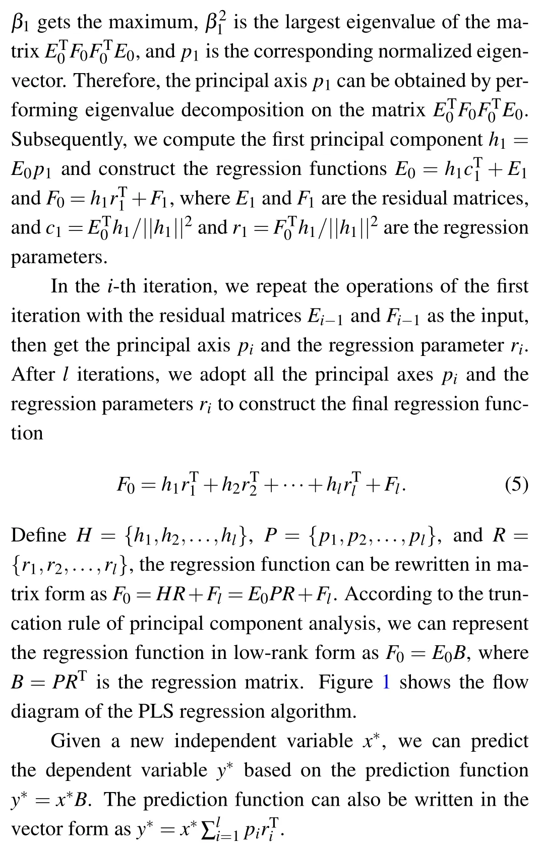
In this section, we briefly review the PLS regression. The kernel work of the PLS regression is to build a linear regression function by projecting independent variables and dependent variables into the new feature space. Based on the linear regression function, we can predict the dependent variable for any independent variable. LetX={x1,...,xm}be the set of the independent variablesxi ∈RnandY={y1,...,ym}be the set of the dependent variablesyi ∈Rw. We centralize and normalizeXandY,respectively,and get the independent variable matrixE0∈Rn×mand the dependent variable matrixF0∈Rn×w. The PLS regression algorithm is an iterative process,and we firstly analyze the first iteration.

Fig. 1. The flow diagram of the PLS regression algorithm, i is the index of the current iteration, variable maxi stores the total number of iterations.

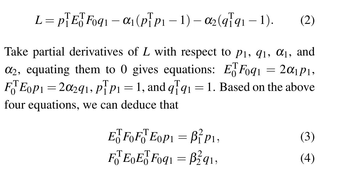
The first work is to find the principal axes(projection directions)p1andq1to create the principal componentsh1andg1such that these two principal components have maximum covariance, whereh1=ET0p1represents the linear combination of the columns ofE0andg1=FT0q1represents the linear combination of the columns ofF0. This work corresponds to the following optimization problem:

where〈,〉means the inner product operation, and||·|| represents thel2norm. Lagrange multiplier method is a way to solve the extremum of multivariate function under a set of constraints. Introducing Lagrange multipliersα1andα2, we transform Eq.(1)into the unconstrained optimization problem

3. QPLS regression algorithm

In this section, we incorporate the design of the quantum eigenvector search method and the residual matrix product method into implementing the QPLS regression algorithm.Firstly,the quantum eigenvector search method is designed to compute the quantum state of the principal axispi. Secondly,the quantum state of the regression parameterriis constructed by combining the quantum eigenvector search method and the inner product operation. Thirdly, the density matrix product method is developed to build the residual matrix productETi FiFTi Ei. Finally, we create a quantum prediction function to predict the dependent variables for new independent variables. Now, we show the implementation process of the first iteration.

3.1. Quantum state preparation

3.2. Quantum eigenvector search method

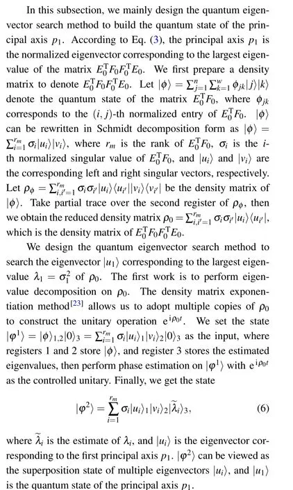
The second work is to extract the eigenvector|u1〉from|φ2〉. QPCA[36]is a quantum principal component analysis method for quantum state tomography. The eigenvectors and eigenvalues can be estimated by measuring the eigenvalue register,and this procedure will be highly efficient when the matrix is low rank. However,the probability of the quantum state of the eigenvalue determines the number of the measurements,so this method would lose logarithmic speed-up when the data set corresponds to an exponentially sizeable high-dimensional matrix. Yu[37]presented another quantum principal component analysis method, which could project high-dimensional data into low-dimensional space,but this method relies on the eigenvalues sorted in descending order. Unfortunately,eigenvalues are stored disorderly in a quantum superposition state,and it is not easy to obtain the ordered eigenvalues.[38]Here,we adopt quantum comparison and amplitude estimation to design a quantum binary search method.This method can extract the eigenvector|u1〉without the ordered eigenvalues and quantum state tomography. The specific process is as follows.

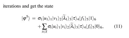
(1) Initialize comparison timesls= log(1/ε), whereεis the error of the estimated eigenvalues. Since all ～λiare in the range (0,1], we initialize the lower boundτmin= 0,the upper boundτmax=1, and the comparison thresholdτ=(τmin+τmax)/2.

(2)Compare the estimated eigenvalue|～λi〉with the comparison threshold|τ〉. We first prepare the initial state|φ2〉|τ〉4|0〉5|0〉6=∑rmi=1σi|ui〉1|vi〉2|～λi〉3|τ〉4|0〉5|0〉6as the input, where register 4 stores the comparison threshold|τ〉and registers 5 and 6 store the comparison result. LetR1represent the comparison operation,which obeys:If|～λi〉is less than|τ〉,set register 6 to|0〉;otherwise,set register 6 to|1〉. After performing the comparison operationR1,we get the state

Figure 2 shows the circuit for a single qubit comparison operation. In this circuit, registers 3 and 4 store|～λi〉and|τ〉,respectively; registers 5 and 6 store the comparison result. If|～λi〉 ＞|τ〉, set registers 5 and 6 to|1〉|1〉; if|～λi〉 ＜|τ〉, set them to|0〉|0〉; otherwise, set them to|0〉|1〉. Figure 3 shows the circuit for thenqubits comparison operation. Similar to the classical comparison circuit, the comparison circuit fornqubits is implemented bynsingle qubit comparison circuits cascading. Let{an,an-1,...,a2,a1}and{bn,bn-1,...,b2,b1}represent the qubit sequences of registers 3 and 4,respectively.This circuit compares the qubit pair(ai,bi)in order from highorder qubit to low-order qubit and passes the comparison result of each qubit pair to the lower-order qubit comparisons.Register 5 contains the qubit sequences{cn,cn-1,...,c2,c1}and{dn-1,...,d2}), which are used to store the comparison results of each qubits pair. Finally, we get the final comparison result from register 6(the qubitd1). Assume|～λi〉and|τ〉are stored in registers 3 and 4, respectively, we perform the comparison operationR1and get the final comparison result:if|～λi〉≥|τ〉,register 6 is|1〉; otherwise,register 6 is|0〉. For the specific design method,refer to Ref.[39].

Fig. 2. Comparison circuit on a single qubit. Reg. 3, Reg. 4, Reg. 5, and Reg.6 represent registers 3,4,5,and 6,respectively. Reg.3 and Reg.4 store|～λi〉and|τ〉,respectively;Reg.5 and Reg.6 store the comparison results.

Fig. 3. Comparison circuit on n qubits. {an,an-1,...,a2,a1} and{bn,bn-1,...,b2,b1} represent the qubit sequences of register 3 and register 4,respectively. {cn,cn-1,...,c2,c1}and{dn,dn-1,...,d2}represent the qubit sequence of register 5,and the qubit d1 represents register 6. All qubit sequences are arranged in descending order. The circuit compares each qubit pair(ai,bi)in order from high-order qubit to low-order qubit and passes the comparison result of each qubit pair to the lower-order qubit comparison.The output of d1 represents the final comparison result.

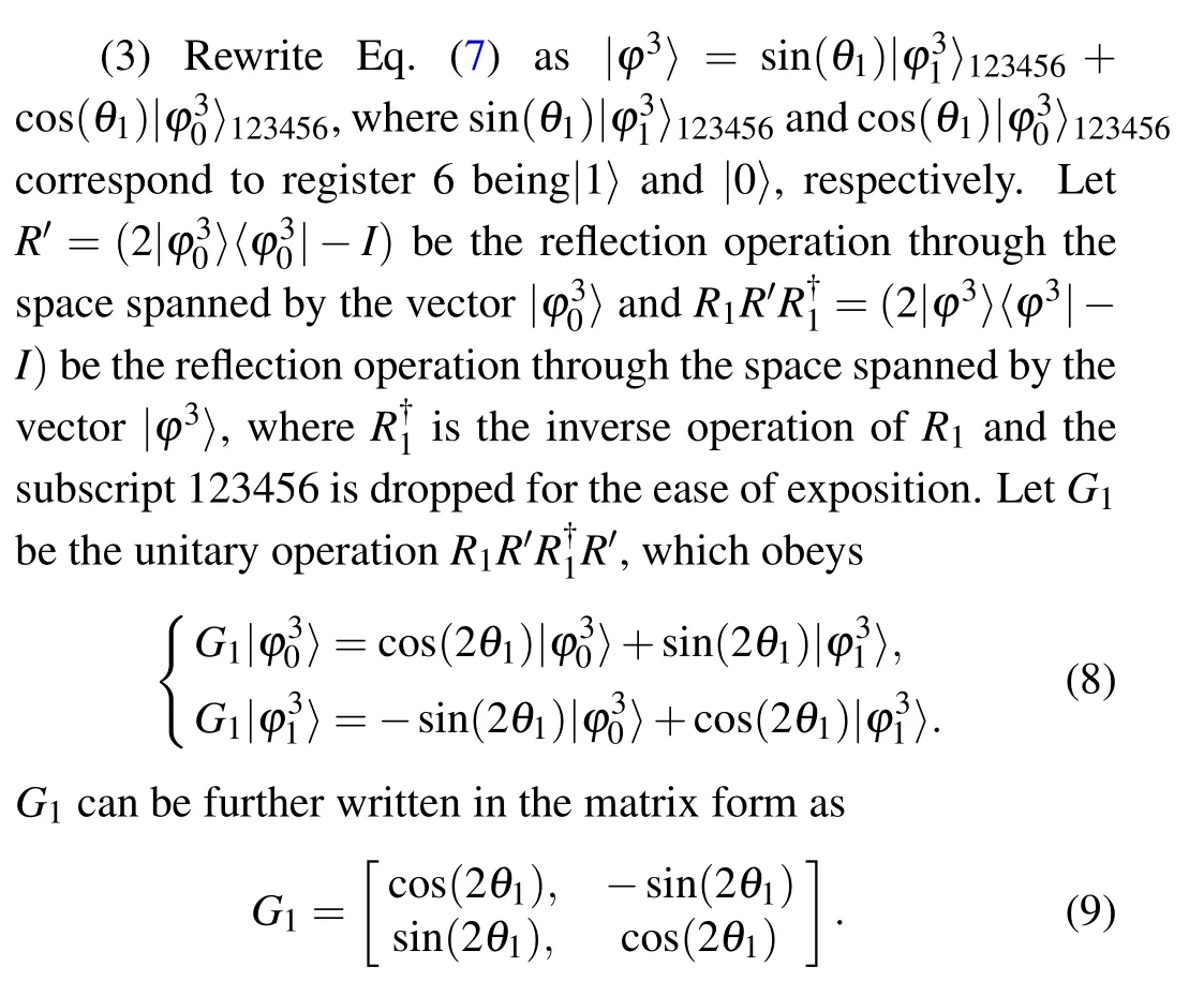
(5) Measure register 6 into|1〉, and remove registers 2,3, 4, and 5. Finally, we get the state|u1〉in register 1, which corresponds to the quantum state of the principal axis|u1〉.It is worth mentioning that amplitude amplification can improve the probability of measurement success quadratically.The quantum eigenvector search method is described in Algorithm 1.

Algorithm 1 Quantum eigenvector search method Input: the quantum state|φ〉for ET0 F0,the reduced density matrix ρ0 for ET0 F0FT0 E0,the iteration times ls.Output: the quantum state|u1〉for the principal axis p1.1: Perform phase estimation on|φ〉and get the eigenvalue decomposition of|φ2〉.2: Initialize i=1,τmin=0,τmax=1,and τ =(τmin+τmax)/2.3: while i ≤ls do 4:Perform comparison operation R1 on|φ2〉and|τ〉and get the comparison result in|φ3〉.5:Act amplitude estimation on|φ3〉to get θ representing the probability of～λi ＜τ.6:If θ ＜0 then 7:Update τmax=τ,and τ =(τmax+τmin)/2 in turn.8:else 9:Update τmin=τ,and τ =(τmax+τmin)/2 in turn.10: i=i+1.11: Measure register 6 with|1〉to get|u1〉corresponding to the principal axis p1.

The circuit of the quantum eigenvector search method is shown in Fig.4,including phase estimation,comparison operation,and amplitude estimation.

Fig. 4. The circuit of the quantum eigenvector search method. Reg. 1-Reg. 7 represent registers 1-7, respectively. The circuit in the first dotted box represents phase estimation,where H means Hadamard transform; eiρ0t represents the unitary operation controlled by eiρ0t;FT+ denotes the inverse operation of quantum Fourier transform. The circuit in the second dotted box represents the quantum binary search operation,R1 denotes comparison operation, and the combination of unitary operations H, G1, and FT+ corresponds to amplitude estimation. The rest dotted boxes represent the repeated quantum binary search operations.

3.3. Construct regression parameters

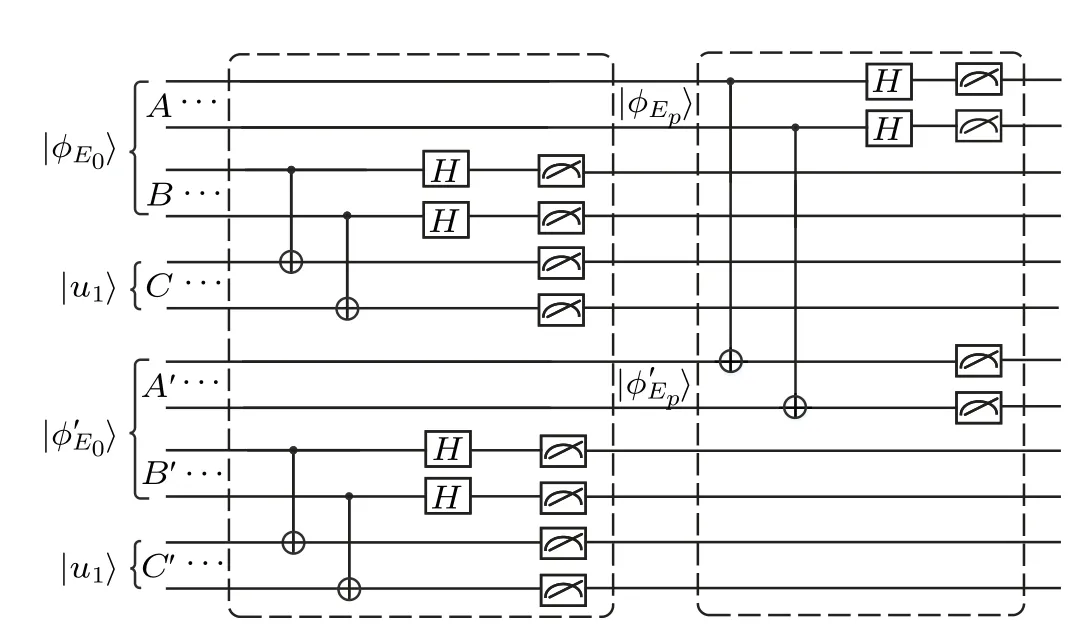
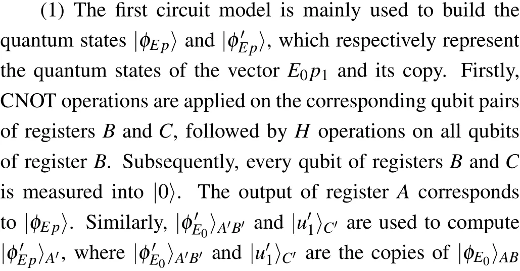
Fig. 5. Circuit of computing ||h1||2. |φE0〉 and |u1〉 represent the quantum states of the matrix E0 and the principal axis p1, respectively. Registers A and B store the quantum state|φE0〉,and register C stores the quantum state|u1〉. Registers A′ and B′ store the quantum state |φ′E0〉, the copy of |φE0〉.Register C′ stores the quantum state|u′1〉,the copy of|u1〉. |φEp〉and|φ′Ep〉are the output of the first circuit model. Two dashed boxes represent two models of the circuit, respectively. The classical post-processing is omitted in this circuit.

3.4. Build residual matrix product

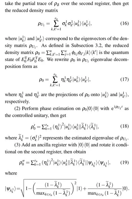
(4)Perform inverse phase estimation and remove the second register. Subsequently, measure the ancilla register into|0〉,and get

Algorithm 2 Quantum density matrix product method Input: the density matrix ρU1 for U1UT1,the density matrix ρ0 for ET0 F0FT0 E0,the number of iterations l.Output: the residual matrix product ρl.1: Iteration i=1.2: while i ≤l do 3:Perform phase estimation on ρi-1 with eiρUit as the controlled unitary and get ρ′i-1.4:Do controlled rotation operation on ρ′i-1 and get ρ′′i-1.5:Perform inverse phase estimation and measurement on ρ′′i-1 and get ρi.6:i=i+1 7: return the residual matrix product ρl.

Figure 6 shows the circuit of building the residual matrix product. The circuit includeslmodels,and thei-th model is used to construct the density matrixρi.

Fig.6. Circuit of building the residual matrix product. The circuit includes l models, where the ith model is used to build the quantum state of the ith residual matrix product. Each module comprises phase estimation PE, inverse phase estimation PE+, and the controlled rotation operation Ry,where phase estimation PE contains Hadamard operation H,the controlled unitary eiρU1t,and inverse quantum Fourier transform FT+. ρi represents the residual matrix product built in the ith iteration. Due to each module has the similar circuit structure, only the first module shows the complete circuit,and the remaining modules are represented by the label eiρUit in the dotted box.

3.5. Prediction

4. Complexity analysis

In this section, we analyze the space and time complexities of the QPLS regression algorithm, which is mainly determined by principal axes computation, building regression parameters,and residual matrices construction.

4.1. Space complexity analysis

In the first stage,we prepare the quantum state|φ〉as the input,which needsO(log(nw))qubits. Letεdenote the error of phase estimation. Phase estimation requiresO(log(1/ε))qubits to store the estimated eigenvalues.[42]Assume amplitude estimation and phase estimation have the same errorε, amplitude estimation needsO(log(1/ε)) qubits to store the estimated amplitudeθ. We get the space complexityO(log(nw/ε2))of the first stage by adding all space complexities together. Forliterations, the total space complexity isO(log(nw/ε2)l).

In the second stage, we first adopt the same operations as the first stage to build the regression parametersr′1; thus,the space complexity isO(log(nw/ε2)). Compared with the first stage,we need to compute the coefficient||E0p1||2further.|φE0〉ABand|u1〉CneedO(log(nm))andO(log(m))qubits,respectively,so the space complexity of calculating||E0p1||2isO(log(nm)+log(m)). Sinceεis very small,O(log(nm)+log(m))can be negligible compared withO(log(nw/ε2)),and the space complexity of this stage isO(log(nw/ε2)). Forliterations,the total space complexity isO(log(nw/ε2)l).

In the third stage,preparation the stateρ0and phase estimation needO(log(nw))andO(log(1/ε))qubits,respectively.Therefore,the space complexity of this stage isO(log(nw/ε)).Since the space complexity of state preparation and phase estimation is the same in each iteration,the total space complexity forliterations isO(log(nw/ε)l).

Table 1 shows the space complexities of the QPLS regression and the PLS regression. Consider thatεis usually very small, the space complexity of the third stage can be negligible. We add all space complexities together and get the total space complexity ～O(log(nw/ε2)l),logarithmic in the independent variable dimensionnand the dependent variable dimensionw.

Table 1. Space complexity.

Finally,we adopt controlled swap test operation to predict the dependent variabley*for the new independent variablex*.Due to|φ*x〉is ann-dimensional vector, the space complexity of controlled swap test isO(log(n)). We need to measure the ancilla resisterO(P(1)(1-P(1))/ε21)times to ensure the errorε1, whereP(1) is the probability that the measurement result is|1〉. SinceP(1)can be viewed as a constant andlcontrolled swap test operations are required,the space complexity of the prediction stage isO(log(n)l/ε21).

4.2. Time complexity analysis

Now, we analyze the time complexity of the QPLS regression. Since the time complexity of preparing the input state|φ〉isO(polylog(nw)), the total time complexity of state preparation isO(polylog(nw)l) forliterations. In the first stage, the time complexity is dominated by phase estimation and the quantum binary search. Phase estimation adopts Hamiltonian evolution[8]to build the unitary operation eiρ0t= eiρ0KΔt.[26]wheretis the evolution time, Δtis the time interval, andKis the number of time intervals. According to Suzuki-Trotter expansion,[23]the error of eiρ0ΔtisO(Δt2), and the maximum error of eiρ0kΔt(k=0,...,K-1)isO(t2/K). Since phase estimation needsKcopies ofρ0and the time to accessρ0isO(polylog(nw)), the time complexity of phase estimation isO(ε-1t2polylog(nw)). The relative error of the eigenvalueλisatisfiesO(λi/t)≤O(λmax/t),whereλmaxrepresents the largest eigenvalue.[43]Since the evolution timetshould beO(1/ε) to ensure the relative error ofO(ε), the time complexity of phase estimation can be further written asO(ε-3polylog(nw)). The time complexity of the quantum binary search is dominated by amplitude estimation. The time complexity of amplitude estimation isO((2+1/2ξ)tG1/ε),[43]wheretG1is the run time ofG1operation, (2+1/2ξ) is a constant determined by the success probability of amplitude estimation. Similar to phase estimation,tG1isO(ε-3polylog(nw)). Amplitude estimation needs to be performedls=log(1/ε)times,thus the time complexity of this stage isO(log(1/ε)ε-4polylog(nw)). Forliterations,the total time complexity of this stage isO(ε-3polylog(nw)l+log(1/ε)ε-4polylog(nw)l).

In the second stage,the time complexity of computing the parameterr′1is the same as the first stage. The time complexity of computing||u1||2is dominated by CNOT andHoperations and can be negligible. Therefore,the total time complexity of this stage forliterations is alsoO(ε-3polylog(nw)l+log(1/ε)ε-4polylog(nw)l).

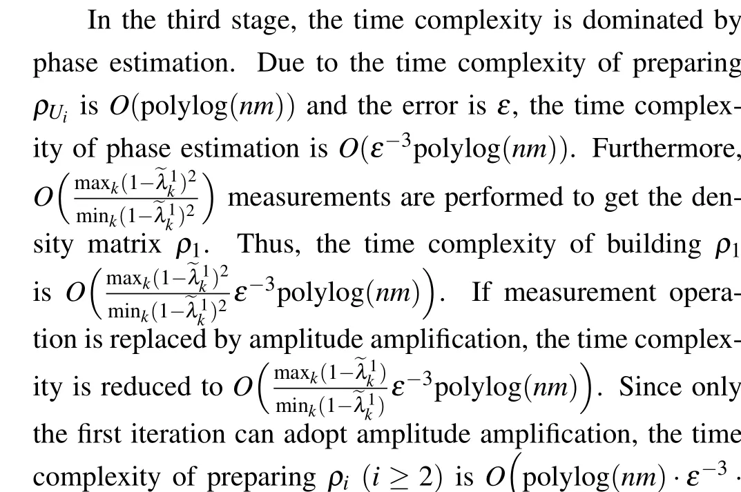
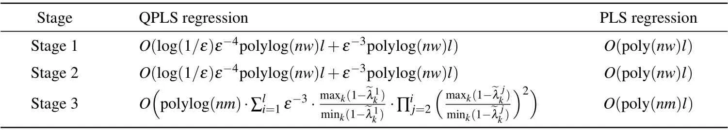
Table 2. Time complexity.

In the prediction stage,the time complexity of controlled swap test operation isO(1), the inner product〈φ*x|ui1〉can reach accuracyε1by iterating controlled swap test operationO(P(1)(1-P(1))/ε21) times, whereP(1) is the probability that the measurement result is|1〉. Therefore, the total time complexity of the prediction stage isO(lP(1)(1-P(1))/ε21).SinceP(1) is a constant, the time complexity can be further written asO(l/ε21),which is determined by the errorε1.

5. Conclusion and future work

Acknowledgements

Project supported by the Fundamental Research Funds for the Central Universities,China(Grant No.2019XD-A02),the National Natural Science Foundation of China (Grant Nos.U1636106,61671087,61170272,and 92046001),Natural Science Foundation of Beijing Municipality,China(Grant No. 4182006), Technological Special Project of Guizhou Province,China(Grant No.20183001),and the Foundation of Guizhou Provincial Key Laboratory of Public Big Data(Grant Nos.2018BDKFJJ016 and 2018BDKFJJ018).