
Review on typical applications and computational optimizations based on semiclassical methods in strong-field physics
2022-03-12 07:44XunQinHuo火勋琴WeiFengYang杨玮枫WenHuiDong董文卉FaChengJin金发成XiWangLiu刘希望HongDanZhang张宏丹andXiaoHongSong宋晓红
Chinese Physics B 2022年3期
关键词:金发
Xun-Qin Huo(火勋琴) Wei-Feng Yang(杨玮枫) Wen-Hui Dong(董文卉) Fa-Cheng Jin(金发成)Xi-Wang Liu(刘希望) Hong-Dan Zhang(张宏丹) and Xiao-Hong Song(宋晓红)
1Institute of Mathematics,College of Science,Shantou University,Shantou 515063,China
2School of Science,Hainan University,Haikou 570288,China
3Research Center for Advanced Optics and Photoelectronics,Department of Physics,College of Science,Shantou University,Shantou 515063,China
4Faculty of Science,Xi’an Aeronautical University,Xi’an 710077,China
Keywords: semiclassical method,attosecond time delay,Phase of Phase,deep learning
1. Introduction
Since the invention of the first laser in 1960s,[1]its rapid development has made it possible to obtain high intensity pulses, which has provided opportunity to study a variety of nonlinear phenomena in strong-field physics. As early as 1965,Voronovet al.[2,3]had already observed the multiphoton ionization (MPI) phenomenon experimentally, that is, electrons can absorb many photons to be ionized. Soon after,Agostiniet al.[4]also observed the MPI phenomenon in experiment. In 1979, the above threshold ionization (ATI) of the xenon atom exposed to an intense laser field was observed for the first time by Agostiniet al.,[5]in which electrons absorb more photons in excess of the minimum photon number necessary to overcome the ionization potential,thus forming a series of peak structures separated by one photon energy in the energy spectrum. In 1987, Shoreet al.[6]predicted the highorder harmonic generation (HHG) and it was experimentally confirmed by McPhersonet al.[7]In the past few decades,the investigation of these nonlinear phenomena had made great progresses, which can be used to not only detect the microscopic particle dynamics process but also reveal the structure information of matter in the strong-field community.[8-25]
The theoretical study of strong-field dynamics can be traced back to the theory proposed by Keldysh,[26,27]Faisal,[28]and Reiss[29](often called as KFR theory), which is widely used to explain experimental phenomena. Based on KFR theory,the various theoretical models considering different effects were developed, such as the well-known strongfield approximation (SFA) method. In 1966, Perelomovet al.[30,31]obtained the ionization rate under the non-adiabatic condition of atomic Coulomb potential system, which is usually called the PPT model. Later, in 1986, Ammosovet al.[32,33]simplified the PPT theory and obtained the electron ionization rate under the quasi-static adiabatic approximation,namely,the ADK model.These theories provide a cornerstone for the later development of a variety of semiclassical methods for strong-field ionization of atoms and molecules.
Here, another early theory involved in the existing semiclassical methods is mentioned. Compared with the Schr¨odinger picture and Heisenberg matrix, Feynman gave a completely new expression of quantum mechanics in his article “Space-Time Approach to Non-relativistic Quantum Mechanics” in 1948, namely the Feynman’s path-integral approach.[34]In this method,the probability of a particle from state A to state B is described as the coherent superposition of the probability amplitude of each path,where the contribution from each path is postulated to be an exponential whose(imaginary)phase is the classical action for the path. It is mentioned that the Feynman’s path-integral method has not changed the quantum mechanical concept of probability.[35]Therefore,the wavefunction obtained by the superposition of all path contributions is equivalent to the result of the Schr¨odinger equation.
It is well known that there are many theoretical methods in strong-field ionization of atoms and molecules, the quantum, classical and semiclassical methods all play an important role in revealing various physical phenomena. The simple classical method is proposed to investigate the subcycle dynamics[36]and the mechanism of physical phenomena such as nonsequential double ionization (NSDI) of atoms.[37,38]Similarly, the quantum method taking timedependent Schr¨odinger equation (TDSE), which is a fully quantum method for the quantitative theoretical simulation has made outstanding contributions in explaining a variety of nonlinear physical phenomena.[39,40]Because of its high accuracy,TDSE result is widely used as a benchmark for evaluating experimental data and other theoretical data.[41-44]However,the TDSE method cannot usually provide an intuitive and transparent physical image. In addition, due to its large computation, TDSE method is always used to the simple atomic or molecular system.
It is impractical to solve TDSE for the multi-electron correlation of complex systems. To provide an alternative approach, compared with TDSE, the semiclassical method has been developed,which can be conducive give a clear physical picture of the strong-field electric dynamics process.
The semiclassical method refers to the classical image to describe the motion of the electron and supplies the classical particles with non-classical phase information. It is derived from the simple man’s model[45,46]in which the strong-field ionization is divided into three-step process: tunneling,acceleration,and collision. It should be emphasized that the semiclassical method presents a clear physical image of the ionization process of atoms and molecules in strong-field ionization,which is helpful to explore the mechanism of some nonlinear physical phenomena.[47]In 1997, Huet al.[48]developed the classical trajectory Monte Carlo (CTMC) model, by considering the transverse momentum distribution of tunneling electrons and the effect of Coulomb potential on the classical trajectories of the ionized electrons. This model had successfully explained the angular distribution structure of highenergy electrons. However,the CTMC method does not consider the interference effect between different ionization paths,which leads to some obvious differences in the quantitative fitting of experiments. To tackle this limitation, in 2014, Liet al.[49,50]developed an intuitive quantum-trajectory Monte Carlo(QTMC)model encoding with Feynman’s path-integral approach, in which the Coulomb effect on electron trajectories and interference effects between electrons with different paths with the same final momentum are fully considered.The QTMC model successfully explains the high-resolution photoelectron angle distribution of ATI,and it was found that the ionic potential plays a significant role in ionization process.[49]It is worth noting that the QTMC uses the quasi-static tunneling rate (ADK model) to describe the first step of ionization. In 2016, Songet al.[51,52]took into account the nonadiabatic effect on the basis of QTMC method and subsequently developed the generalized quantum-trajectory Monte Carlo(GQTMC)method. The GQTMC approach can be used to obtain the momentum distribution for different polarizations of the laser field and wide range of Keldysh parameterγ. The GQTMC method has achieved great success in studying ionization process for the deep tunneling region and revealing the mechanism of side lobes[53]in both adiabatic and non-adiabatic regions.[54,55]
Another branch of semiclassical methods is a series of SFA methods developed based on KFR theory. In the SFA,the plane-wave Gordon-Volkov state,[56,57]which is is used to approximate the continuous state to simplify the transition process from the ground state to the continuous state. It is noted that in SFA, the interaction between electrons and the Coulomb potential is ignored. Therefore,the results are difficult to be fully quantitatively consistent with the experimental or TDSE results. To tackle this problem, the different correction methods to improve the SFA model were developed.One of the common corrections is Coulomb-Volkov approximation (CVA)[58,59]which uses Coulomb-distorted wave replaced by plane wave. In 2008, Popruzhenkoet al.[60]developed Coulomb-corrected SFA (CCSFA) method by taking the perturbation Coulomb effect into the action of SFA to correct the phase, in which the electron trajectory is not affected by the Coulomb potential. Subsequently, based on the CCSFA,Yanet al.[61,62]developed trajectory-based Coulomb SFA (TCSFA), by considering the influence of Coulomb potential on the motion of electrons in continuous state. Generally, there need to be hundreds of millions of trajectories for both CCSFA and TCSFA in calculations to get relatively clear physical picture, while the Coulomb quantumorbit strong-field approximation (CQSFA) is an exception as it only needs a few contributed trajectories for each value of the final momentum.[63-65]
This review starts with the semiclassical method based on Feynman’s path-integral. On this basis, we focus on the important applications of semiclassical methods in trajectory analysis and information extraction. The rest of this paper is organized as follows: in Section 2, we will briefly introduce some semiclassical methods commonly used to deal with laser-matter interactions.In Section 3,we will mention the application of semiclassical methods to analyze the underlying physical mechanisms of interference structures. In Section 4,we present some examples of attosecond time extraction by semiclassical methods. Then in Section 5, we show some time-saving optimizations for semiclassical calculations. At last,we will summarize in Section 6.
2. Theoretical method
There are many semiclassical methods in strong-field physics,such as QTMC,TCSFA,CQSFA,etc.,whose detailed description can be seen in Refs.[66,67].In this review,we will mainly introduce the GQTMC and CCSFA methods.
2.1. GQTMC method
GQTMC method is based on the nonadiabatic ionization theory,[30,31]classical dynamics with combined laser and Coulomb fields,[48,68]and Feynman’s path-integral approach.[49,69]The ionization rate is given as
Following ionization, the evolution of the electron wavepacket is simulated by launching randomly a set of electron trajectories with different initial conditions. The classical motion of an electron in the combined laser and Coulomb fields is governed by the time-dependent Newton equation(TDNE)
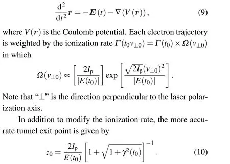
Here,γ(t0)is the Keldysh parameter depending on the instantaneous time. It is noticed that the exit point shifts toward the atomic core due to the nonadiabatic effect. According to Feynman’s path-integral approach,the phase of thej-th electron trajectory in the ensemble is given by the classical action along the trajectory[49,69]

2.2. CCSFA method
Compared with SFA,[70]the effect of Coulomb potential on the ionized electron is considered in the CCSFA approach.Hence this method has a wide range of applications in strongfield physics.
The Hamiltonian of an atom coupled to the timedependent external field, which is described by an operatorHI(t),is given by
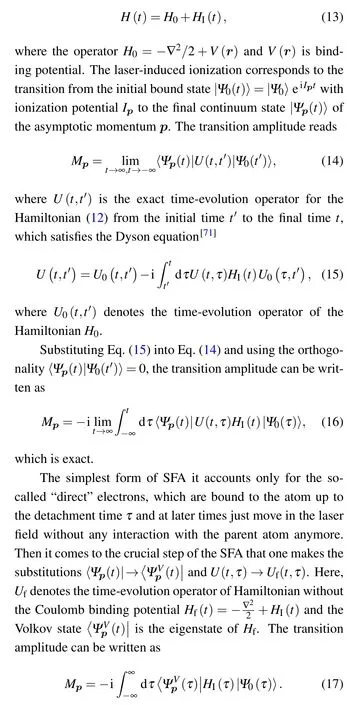
Here, fort <τ, the electron is bound to the atom its interaction with the laser field can be ignored.At timeτ,it is ionized,and fort >τ,the electron motion is driven by the intense laser field without the influence of the binding potential.
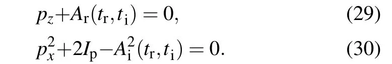
The first term in the above equation is the phase contribution of the subbarrier imaginary part,i.e., the quantum tunneling process, the second term is the phase contribution from the evolution of electrons in real time space.
3. Trajectory information extraction based on semiclassical method
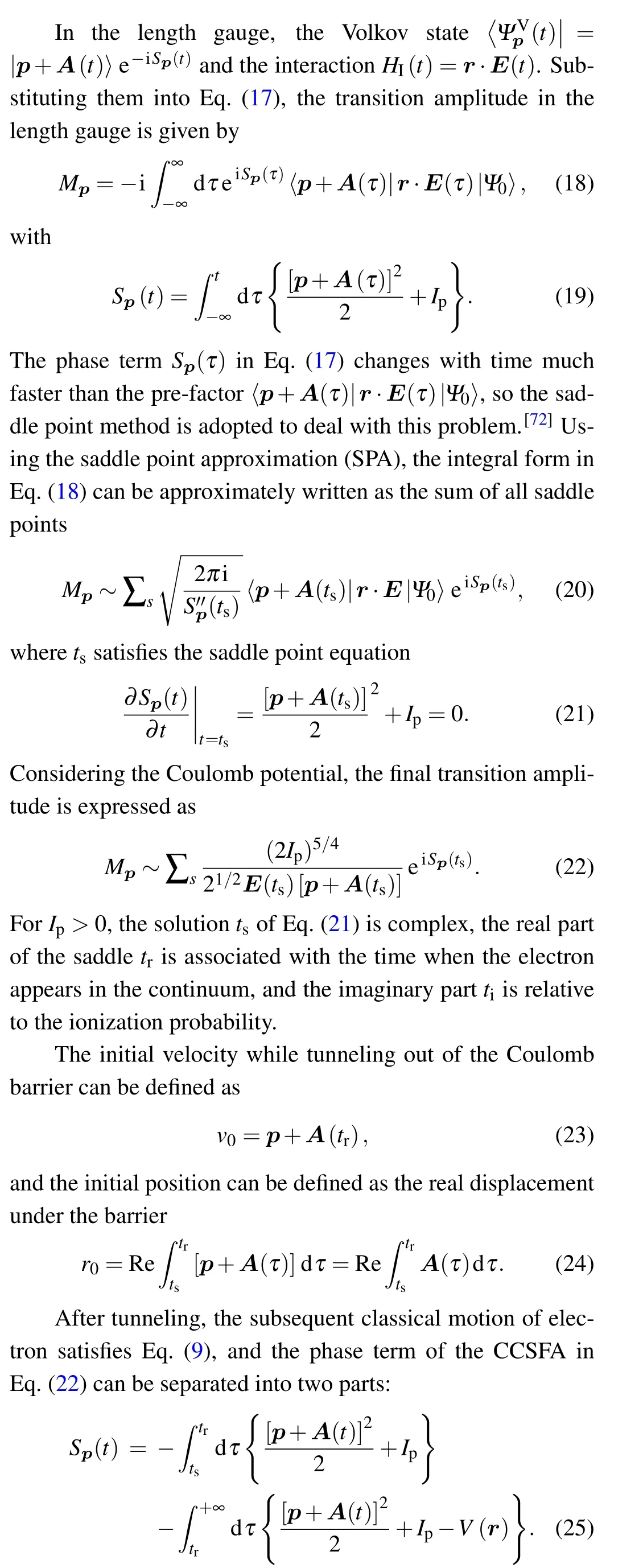
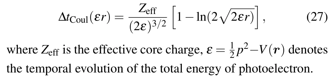
In the previous section, we introduced several typical semiclassical methods that are widely used in strong-field physics. The photoelectron momentum distribution (PMD)is formed by the interference of electrons, so it encodes rich spatiotemporal dynamic information. The semiclassical methods can be in favor of extracting the information of specific interference structure and revealing electronic dynamics process.[73,74]In the tunneling theory, the ionization rate of atoms and molecules depends exponentially on the intensity of the instantaneous laser field.[75]Therefore, in the periodic oscillating laser field,the ionized wavepackets are formed near the electric field maximum. These ionization wavepackets interfere with each other and form various interference structures. The common interference patterns in PMDs include spider,[76]carpet,[77,78]fan,[79,80]and fork shapes,[81]etc. In Ref. [82], the PMDs of argon atom and N2molecule show different interference patterns in different energy ranges. By the analysis of electron trajectories, the PMD is attributed to different trajectories, which can be roughly classified as four groups, as shown in Fig. 1(a). For type-I trajectories (black line), the electron moves directly to the detector after ionization,without returning to the parent core.For type-II and type-III trajectories (green, blue, and gray lines), the electron first moves away from the detector and then turns around and finally arrives at the detector. For type-IV trajectories (purple line),the electron initially moving to the detector goes around the core and finally moves toward the detector again. Surprisingly,it was found that the interference patterns of fan,spider,and carpet structures are contributed by the interference of trajectories I+II(see Fig.1(b)),II+III(see Fig.1(c)),and III+IV(see Fig.1(d)),respectively.
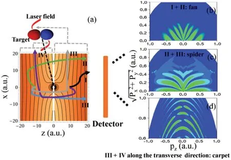
Fig.1. (a)Schematic diagram of the dominant trajectories, classified from I to IV.(b)-(d)The interference patterns in the final photoelectron momentum distribution of contributions of trajectories in panel(a). Adapted from Ref.[82].
Recently, Songet al.[54]reconstructed the experimental PMDs of argon atom exposed to an 800-nm laser pulse with intensity of 1.7×10¹⁴W/cm2. In addition to the universal holographic interference stripes,which are almost straight,arc shape structures are also observed. In the theoretical simulation,both the TDSE and GQTMC methods can well reproduce the conventional holographic and curved stripes in experimental results.
In the following,we will focus on the semiclassical analysis of curved interference patterns. Figure 2(a) shows the PMD simulated by the GQTMC method, where the straight holographic interference fringes and curved stripes are marked by solid and dashed lines, respectively. To gain more insight into the origin of the curved interference structure, all electron trajectories contributing to the momentum spectrum with final longitudinal momentum in the rangepz ≫0.3 a.u. was analyzed. In this region,both holographic fringes and curved interference fringes can be clearly seen. Figure 2(b)shows the distribution of the initial tunneling phase and initial transverse momentum of the trajectories contributing to this momentum range. One can see that, the initial conditions of the electron within one laser cycle are separated into four areas,which are marked as A,B,C,and D.For each area,the initial conditions are different,so the corresponding electron trajectory types are also different.
Figure 2(c) shows the typical electron trajectories from areas B in Fig.2(b). Obviously,there are two types of electron trajectories in the B area of Fig. 2(c). The black lines represent the trajectories of electrons with small initial transverse momenta, which are formed because of forward scattered by the ionic potential in the direction of laser polarization. While the red lines represent the trajectories of electrons with large initial transverse momenta,which only revisit and pass by the core at large distances without scattering and are therefore considered direct electrons. To identify contribution of two types of electron trajectories to the total momentum spectrum,only the electron trajectories in area B are first extracted and the final PMD is reconstructed. In the reconstructed PMD,there are only straight and radial interference structures,which correspond to the interference fringes marked by solid line in Fig.2(a).This result indicated that electrons emitted from area B do not result in curved structures.
Figure 2(d) shows typical electron trajectories in area A and their contributions are analyzed. The reconstructed PMD contain an obvious curved structure, which means that the electrons in area A are the source of the curved interference structure in Fig.2(a). At first glance,the electron trajectories of the electron in Fig. 2(d), marked in red and green respectively, look basically the same, but there are obvious differences in details, especially aroundz=0. The enlargements of electron trajectories are shown in Figs. 2(e) and 2(f). As more clearly shown in Fig. 2(e), the Coulomb field pulls the electrons back aroundz=0 along the laser polarization and then backward scattering in the direction perpendicular to the laser polarization axis. This kind of special rescattering that causes the curved interference structure is called “Coulomb field-driven transverse backward scattering”. Moreover, this Coulomb-field-driven transverse backward scattering may occur not only at the first return(see Fig.2(e))also at the second return(see Fig.2(f)).
As mentioned above,the semiclassical method has an advantage in analyzing the multifarious interference structures,which is reflected in the extraction of trajectory information.It is mentioned that the semiclassical method can be also used to extract attosecond time of photoelectric emission. We will discuss some applications of semiclassical method in extracting attosecond time in Section 4.
Fig. 2. (a) PMD simulated by GQTMC method. (b) Distributions of the initial transverse velocities and the initial ionization phases. The color code denotes the weights of the electrons in areas A-D.(c)-(d)Typical trajectories of electrons in area B(c)and in area A(d). (e)-(f)Enlargements of electron trajectories scattered at the first and second returns in panel(c). Adapted from Ref.[54].
4. Application of semiclassical method to extracting photoelectric emission time
4.1. Phase of phase
Momentum photoelectron spectra of atoms and molecules in an intense laser field carry rich ultrafast dynamics information,and it is of great significance to reveal this information. It has been proved by many pump-probe experiments that the dynamic information in photoelectric emission can be extracted by adjusting the carrier-envelope phase (CEP) of a monochromatic field or the relative phase between two-color laser fields.[83-85]In fact, as early as 1994, Schumacheret al.[86]found that the electron yield in a two-color laser field is modulated by the relative phase. In 2014, Zippet al.[87]detected the inherent delay of ATI by modulating the relative phase and processed experimental photoelectronic signals by using an asymmetric degree fitting method. It is worthwhile mentioning that this asymmetric degree fitting method is essentially a Fourier analysis.[88]Subsequently, Skruszewiczet al.[89]developed the phase of phase method, which takes the photoelectron yield as a function of the relative phase. In this process,electrons are first ionized by a strong fundamental frequency field and then a weak double frequency field is added as a perturbation to detect the motion of electrons after ionization.[88]By modulating the relative phasesφ, the specific ionization channels can be selectively enhanced or suppressed.[90,91]More importantly, the associated structure and its dynamics information can be encoded in the photoelectron momentum spectrum of each determined relative phase.
When the relative phaseφchanges, the photoelectron yieldY(p,φ) at each momentumpcan be characterized by two functions ofp, namely, the relative phase contrast (RPC(p)) and phase of phase (PP(p)).[89]Generally,RPC and PP can be quickly determined by fast-FouriertransformingY(p,φ)with respect toφfor eachp. If only the first-order terms in Fourier analysis are considered, the photoelectron yieldY(p,φ)behaves predominantly asY(p,φ)=RPC(p)·cos(φ+PP(p))+C, where RPC and PP represent photoelectron yield periodically modulated by the relative phase of the dichromatic field and the phase of the signal itself, respectively.[92]The phase of phase method can be used to not only extract temporal information from the photoelectron momentum spectrum,but also has great potential in analyzing interference structures. In 2017,Almajidet al.[93]studied the ATI of xenon atoms from both theoretical and experimental aspects in the condition of the two-color linearly polarized laser fields and deduced the first-order Fourier component with the strong-field approximation method. In 2016, Natanet al.[88]also measured the relationship between the electron yield and the relative phase of the two-color laser field,and the results were basically consistent with those in Ref.[86]. Further, the second order component in Fourier analysis is considered, where the fitting relation isY(p,φ) = RPC(p)2ω ·cos(φ+PP(p)2ω)+RPC(p)4ω·cos(φ+PP(p)4ω).The first and second order Fourier components of RPC(p) and PP(p)can be decoupled into the contribution of direct and scattered electrons to the photoionization process.[88]
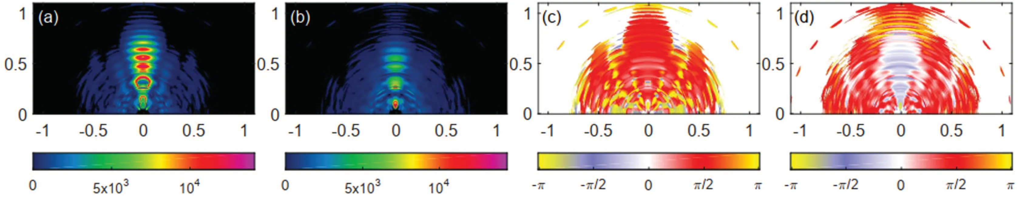
Fig.3. The spectrum obtained by Fourier analysis. Amplitudes RPC(p)2ω (a)and phases PP(p)2ω (c)as a function of momentum components px(horizontal axis)and py(vertical axis)of the Fourier coefficient that corresponds to frequency 2ω.The amplitudes RPC(p)4ω (c)and phases PP(p)4ω (d)of the Fourier component at 4ω. Adapted from Ref.[88].
In general,the frequency ratio of the two-color laser field used in the phase of phase method is 1:2. Tulskyet al.[94]extended the frequency ratio to arbitrary frequency and distinguished the incoherent scattering generated by multiple scattering of neutral helium atoms. They also found that the RPC and PP spectra have triple symmetry under the circularly polarized field.[95]In terms of extracting time information,Poratet al.[91]successfully separated the contribution of two signals in photoelectron hologram and found that the difference in ionization time between the two signals was only a few tens of attoseconds. W¨urzleret al.[92]studied the effect of superposition of multiple electrons caused by heavy scattering on the reconstructed ionization time.
Recently, Songet al.[96]proposed a spectral solution method, namely, combining the phase of phase method with the semiclassical GQTMC method.This approach can be used to extract attosecond time information of photoelectric emission. Here, we will focus on this spectral method of extracting time information. As in the experimental observation and theoretical simulations, the PMD is obtained by using a twocolor laser pulse with strong pump and weak probe fields. By changing the relative phaseφLof the two-color fields from 0 to 2πat a step size of 0.05π, the 40 different PMDs containing ATI and sideband(SB)structures(see Fig.4(a))were obtained. For each ATI and SB peaks, the fitting formula for the dependence between the photoelectron yieldYnand the relative phaseφLisYn(φL) =Y0+A0cos(φL+Φn), hereY0,A0,andΦnare the zero-frequency component,contrast amplitude, and fitting phase, respectively. The fitting time delay isΦn/ω. For analysis, the typical PMD of then-th ATI or SB peak withφL=Φncan be chosen, which means that photoelectrons of then-th ATI or SB peaks have the maximal yield(see Fig.4(b)). Then,the normalized photoelectron probability as a function of initial conditions for then-th ATI peak can be used to analyze the spatial-temporal dynamics behind the measured time delays(see Fig.4(c)).
The dynamic process of sub-cycle photoelectron emission can be observed in attosecond scale by using the phase of phase method combined with GQTMC,which will help us to explore the most fundamental problem in strong-field physics and quantum mechanism, namely time. In the following, we will introduce some typical works of time extraction in strongfield computation.

Fig. 4. (a) Extracted phase of the phase. (b) The PMD with φL =Φn. (c)Probability distribution of the initial conditions of photoelectrons contributing to the n-th ATI peak in the PMD with φL=Φn. Adapted from Ref.[96].
4.2. Attosecond time delay of retrapped resonant ionization
In recent years, the research of extracting structural information from strong field observables capable of providing time-resolved imaging of ultrafast processes in the attosecond scale has attracted much attention.[97-99]For example, Zhouet al.[100]have proposed a method that enables one to extract complementary structural information represented by the phase of the scattering amplitude in the near-forward direction. In addition, strong-field tunneling ionization is the initial step for various ultrafast dynamics in intense laser-atom and molecule interactions. Time-resolved tunneling ionization is essential for an accurate understanding of these ultrafast processes and for achieving ultimate accuracy in attosecond metrology.[101,102]
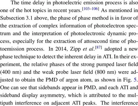
Fig.5. Photoelectron momentum spectra at the relative phase of two laser fields of(a)φ =0; (b)φ =π/2; (c)φ =π. Laser polarization of both colors was along the vertical axis. Insets display the relative delay of the optical fields. Adapted from Ref.[87].

Fig.6. 2D spectra of energy versus relative phase φL of the two-color laser fields simulated by the experiment(a)and the GQTMC method(b).Adapted from Refs.[87,96].

Fig. 7. Retrieved time delays of ATI and SB peaks from the experiment,TDSE,and GQTMC simulations. Adapted from Ref.[96].
In 2018, Songet al.[96]used a semiclassical method to well replicate two-dimensional (2D) spectrum of energy obtained by Zippet al.[87](see Fig.6). Moreover,a spectral solution method combining GQTMC and phase of phase methods was introduced,[96]which was described in detail in Subsection 4.1. Then, by using statistical quantum orbits, ultrafast dynamic time information can be obtained by spectral solution. In the calculation, both TDSE and GQTMC method are used to investigate the time delays in ATI. Through the above fitting method,π ≈667 attosecond (as) out of phase is obtained between all ATI and sideband (SB) peaks without the atomic potential. When the atomic potential is considered in GQTMC simulation,the results are in good agreement with that of both the experiment and TDSE.Comparing with the case without the atomic potential,there is a large positive phase deviation in the 1st ATI peak and a small negative phase deviation in the 5th ATI peak and nearly no deviation for other ATI peaks,as shown in Fig.7.
To further explore the underlying physics of phase shift in ATI spectrum,it is indispensable to analyze the photoelectron probability distribution and its corresponding trajectories.Figures 8(a)-8(c) are the normalized photoelectron probability as a function of initial velocity|v0| and initial ionization phaseωt0for the 1st, 3rd, and 5th ATI peaks, respectively.As can be seen from Fig.8(a),the photoelectrons contributing to the 1st ATI peak come from four parts, in which parts A and B are scattered electron trajectories, while parts C and D are the direct electron trajectories. Figures 8(d) and 8(g) are typical of trajectories from part A and its corresponding temporal evolution of the total energy of photoelectron. Evidence of the photoemission time delay can be easily found by looking at the electron trajectories in Fig. 8(g),i.e., the electron is transiently re-trapped by the Coulomb field into a negative energy state and is eventually released with a positive final energy once the sufficient energy is obtained. This kind of time delay caused by atom potential induced re-trapped resonant scattering (RETRS) is a prototypical case of the EWS delay.Figures 8(f) and 8(i) are the analysis of electron trajectories in part B,in which besides the RETRS,there also exists rapid hard collision. As can be seen from Fig.8(a)to Fig.8(c),the A part of the 3rd and the 5th ATI almost disappears,which further proved that the significant phase shift of the 1st ATI was attributed to RETRS.From the above analysis,we can draw a conclusion that the RETRS retarding an electron for a positive time delay and the hard collision contributes to a negative time delay(see Fig.8(c)).

Fig.8. The initial conditions and photoelectron probability distributions of(a)1st,(b)3rd,and(c)5th ATI peaks,respectively: (d)and(e)the typical trajectory of electrons in part A;(f)the typical trajectory of electrons in part B;(g)-(i)the corresponding temporal evolution of the total energy of the photoelectron shown in panels(d)-(f),respectively. Adapted from Ref.[96].
The relative time delay of the direct electrons and the scattered electrons is calculated by using the statistical average method. By distinguishing the trajectories of the direct electrons and the scattered electrons and recording their weights,the expected value of the total time delay can be expressed as

Here,Wd(i),Wsc(i), ˜td, and ˜tscare the weights and the expectation values of the time delay for the direct and scattered trajectories, respectively. According to Eq. (26), the expectation value of the time delay of the direct electron and the scattered electron areπand 1.59π, respectively, so the relative time delay between the scattered and direct electrons contributing to the 1st ATI peak is ˜tsc-˜td≈0.59π ≈394 as. In the same way, the relative time delay for the 5th ATI peak is-0.1π ≈-67 as.
In fact,the EWS time delay is the energy variation of the partial wave scattering phase shift at short-range potential. If considering the Coulomb distortion caused by the interaction between the emitted electron and the long-range Coulomb potential, the Coulomb correction of the EWS delay can be expressed as[107,108]
The results obtained above unify the quantum EWS time delay and classical Coulomb-induced time delay.More importantly, it provides a new perspective for the detection of high time-resolved attosecond time delay,which is of great significance. Just as the Ref. [109] says “Theoretically, the origin of the time delays measured by the multiphoton technique has been traced to retrapped resonant ionization and the different numerical values of the time delays compared to those measured by the RABBIT technique have been given”.
4.3. Freeman resonance delay
In 1987, Freeman resonance phenomenon was first discovered experimentally.[110]When xenon atoms are exposed to the pulses at 616 nm ranging from 15 ps to 0.4 ps, it was found that the low-energy ATI peak is split into several fine structures at pulse widths less than 1 picosecond. Each subpeak of the low-energy part in the energy spectrum is attributed to the resonance from the ground state to an excited state. Recent studies have predicted that two-photon ionization of helium has a significant emission delay when it comes to the resonant intermediate state,but the physical mechanism causing resonance and the specific time of the photoelectron in the excited state are still open questions.[111]In 2017,Gonget al.[112]observed a Freeman resonance delay of 140±40 attoseconds between the photoelectrons emitted via the 4f and 5p Rydberg states of argon by comparison between experiments and GQTMC theoretical simulations.
Experimentally, a phase-controlled orthogonal two-color(OTC) femtosecond laser pulse with comparable fundamental field and its second harmonic was employed to observe the spatial- and energy-resolved photoelectron angular distributions(PADs),which is a function of the relative phaseφLof the OTC field.Figure 9(a)shows the experimentally measuredφLintegrated PAD and Fig.9(b)is the corresponding theoretical simulation result. As you can see that the GQTMC simulation well reproduces the main features of the experimental PAD. It is worth noting that the interference structure in the PAD varies with the emission angle in Fig.9(a). Forφe=0°,only ATI (labeled by white dots) structure appears; while forφe=30°, besides ATI structure, sideband (labeled by black dots)structure also appears.
Fig.9. (a)Measured PAD and (b)simulated PAD integrated over φL. The fundamental field and its second harmonic of the OTC field have comparable intensities,which are both estimated to be 8.5×10¹³ W/cm2 in experimental measurement and theoretical simulation. Adapted from Ref.[112].
Figure 10 shows the relationship between experimental and theoretical results of electron energyEeand relative phaseφLat different range of electron emission angles,where the experimentally measuredφL-Eespectra are given by Figs.10(a)and 10(e), and figures 10(b) and 10(f) are the corresponding normalized spectra. By fitting the normalized spectrum with the formulaYN(φL) =Y0+A0cos(φL+φPP) for each ATI peak, the contrast amplitudeA0(red dashed curves in Figs. 10(c) and 10(g) andφPP(Figs. 10(d) and 10(h))) of the photoelectron energy spectra is retrieved. As can be seen from Figs.10(d)and 10(h),theφPPof the sidebands1is-1.53πand its adjacent main peaksm1andm2are-0.69πand-0.63π,respectively. Interestingly, these two peaks correspond to the bright signal aroundpy=0.33 a.u. in Fig.9(a)and the sharp peaks at 1.75 eV and 2.18 eV in Fig. 10(a). This result indicates that the two peaks are the photoelectrons emitted via the Freeman resonance[110]of the field-dressed 5p and 4f Rydberg states of argon.[113,114]
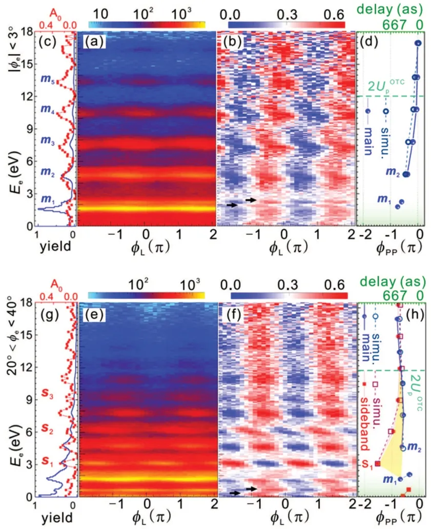
Fig. 10. (a), (e) Measured and (b), (f) normalized 2D spectra of Ee versus φL. (c), (g)Measured φL-integrated Ee distribution(blue solid curves)and retrieved contrast amplitude A0 (red dashed curves). (d), (h) Retrieved phase-of-phase φPP of main(blue solid circles)and sideband peaks(red solid squares). Adapted from Ref.[112].
The attosecond time delay due to Freeman resonance was calculated by using the spectral resolution method mentioned in Subsection 4.1. For each pathway, the time delay of the photoionization includes the contributions from the multiphoton transition process,the propagation of the photoelectron in the combined field of the atomic potential and the laser field,and the Freeman resonance delay. In the GQTMC simulation,the Freeman resonance is not able to be included while other processes can be well described. However, both the experimental and TDSE results include the Freeman resonance, as well as other processes already covered by the GQTMC simulation. The Freeman resonance delay of the photoelectrons emitted via the field-dressed 4f and 5p states can be obtained by using the formula
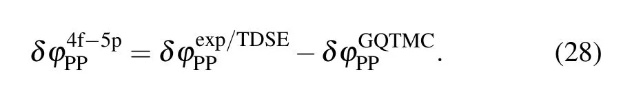
The following table gives the calculation results when the emission angles are 0°and 30°respectively.
As you can see from Table 1, Freeman resonance time does not depend on the emission angle,and the averaged phase difference is(0.19π+0.21π)/2=0.205π,which corresponds to a difference of 140 as of the Freeman resonance delay between the photoelectrons emitted via the 5p and 4f states.
Table 1. Experimentally measured and simulated phase differences between two photoionization pathways,photoelectrons emitted via the 4f and 5p states of argon. Adapted from Ref.[112].
5. Optimal calculation of semiclassical method
Both CCSFA and GQTMC are semiclassical methods,which are developed based on Feynman’s path-integral. The result of Feynman’s path-integral can be expressed as the coherent superposition of all possible space-time path contributions, which can well reproduce the quantum wavefunction and its corresponding time evolution.[34,35,115]Although these semiclassical methods have incomparable advantages in explaining the formation of the interference structures in PMDs,a great deal of time is consumed in the calculation of hundreds of millions of trajectories. Especially for CCSFA method,there are a lot of inevitable numerical iterations in the solution process,which takes up too much time and leads to low computational efficiency.[60-62,116]More importantly, compared with increasingly sophisticated experiments, these semiclassical methods have been limited in terms of explaining some new quantum phenomena and obtaining high-resolution photoelectron spectra due to their limited number of paths.
For the original CCSFA method, the most timeconsuming step is to find the solutiontsof the saddle point equation for a mass of the initial ensemble. Apparently,tsis the complex number. The electron undergoing from complex timetsto real timetrshows the process of tunneling under the barrier. After tunneling out at real timetr, the motion of electron would be regarded as the motion of classical particles driven by an external field and the Coulomb potential,whose initial conditions are obtained by saddle points.
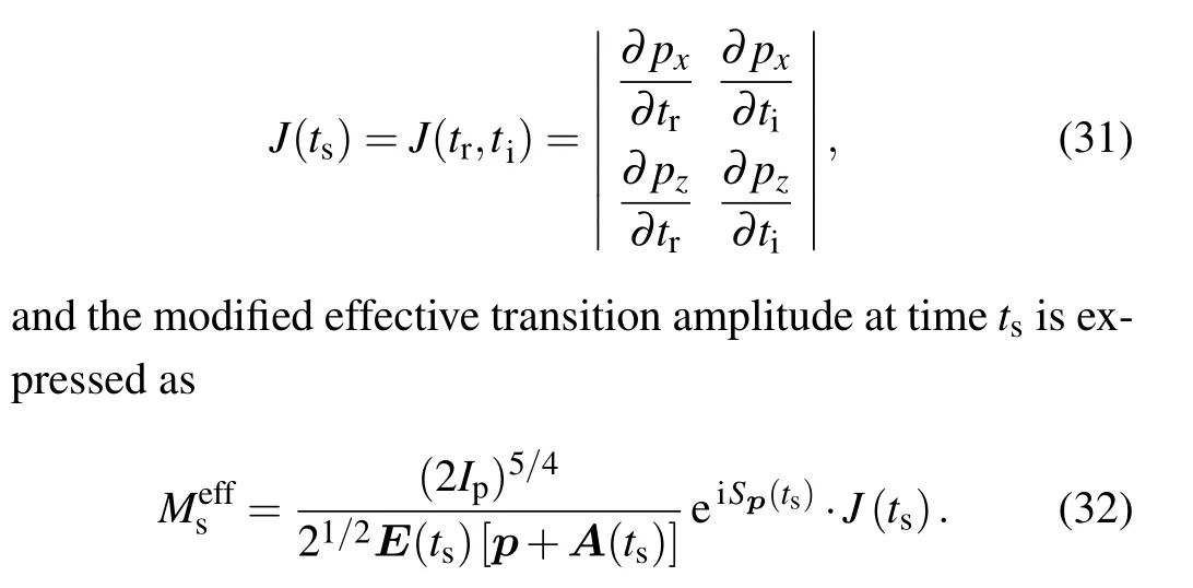
Recently, there has been a lot of research on improving the performance of CCSFA methods from different approaches.[117-119]Xiaoet al.[118]presented an alternative time-sampling scheme to overcome the time-consuming problem. In this method, the given initial random samples are no longer momentum (px,pz), but random saddle point solutionts= (tr,ti). Thus, the vectorAzof the specific laser pulse should be a complex function asAz(tr,ti)=Ar(tr,ti)+iAi(tr,ti). Then the saddle point equation(20)can be derived into the following algebraic equations:[118]
The solutions (px,pz) of the above two equations can be expressed analytically by the sample solutionts=(tr,ti). The initial conditions for classical motion can also be written as the function (tr,ti). Therefore, the time-sampling method eliminates the requirement to solve the saddle point equation,which saves the computational consumption by tens of times.It is worth noting that the final state momentum distribution obtained by the original CCSFA method is uniform in its sampling momentum space(px,pz), while the time-sampling method samples in the time plane (tr,ti), which leads to uneven sampling in the momentum space(px,pz). The essential reason for this result is that the mapping between momentum and time is nonlinear. Therefore, it is necessary to introduce a Jacobian matrixJ(ts) between the time and momentum to modify Eq.(21)and get the correct result of the transition amplitude,where Jacobian matrix is written as
The 2D PMDs of hydrogen atom obtained by the original CCSFA and timesampling method are shown in Fig.11.In the calculation,multicore parallelization is adopted. For the original CCSFA method, the consumed time is divided into two parts: solving the saddle-point equations and the propagation of electron in classical region. According to the statistics,the two processes take 57.5 min and 5.2 min respectively in dealing with one million electrons per core. While with the timesampling method, the whole calculation process only spends 3.5 min. For long pulse, the time saving advantage of time sampling method will be more obvious. Therefore, the timesampling method can not only well reproduce the original calculation results of CCSFA method,but also save tens of times of the calculation time. This will provide a good way to solve the complex computation problem in strong-field physics.
In recent years, deep learning (DL) has attracted worldwide attention and has been applied in many fields.[120-124]In 2020, Liuet al.[119]introduced the deep learning performed strong-field Feynman’s formulation (DLPSFFF), which has been shown wondrous capacity and high efficiency in processing massive data in strong-field physics.
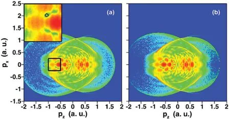
Fig. 11. The 2D photoelectron momentum distributions of hydrogen atom is obtained by(a)CCSFA method and(b)time-sampling method. A 4-cycle linearly polarized laser pulse at wavelength of 800-nm and peak intensity of 1×10¹⁴ W/cm2 with a cos2 envelope is used in the calculation. Adapted from Ref.[118].
In the DLPSFFF approach,a very small number of sample trajectories is used for training and a prediction tool is built, then the built prediction tool is used to calculate a series of arbitrary trajectory and give the final prediction results.
In general, deep neural networks (DNNs) is used in DLPSFFF approach to encode the space-time dynamics information in photoemission and find a unified mapping relationship between initial and final states for different types of space-time paths. As can be seen from the schematic illustrations of DNN in Fig.12,it is divided into three layers,namely the input layer, the hidden layers and the output layer. Here,it is important to note three hidden layers with 250 neurons in each layer are adopted.However,the direct and scattered electron trajectories in different dynamic processes are mixed up in the set,which leads to the diversity of data,so it is difficult to accurately find the mapping between input data and output data using DNNs alone. To overcome this challenge, a fully connected multilayer feed forward network, known as multilayer perceptron (MLP), with three hidden layers was constructed to classify the data of direct and scattered trajectories.Thus,assisted by MLP to pre-classify data of electron trajectories, the DNNs can be trained with only input and output data of few available sample trajectories, without knowing in advance the detailed dynamics of the sample trajectories,and then create a predictive tool that directly predicts the final results of arbitrary trajectory given its initial conditions.
The following,taking CCSFA as an example,briefly describes the calculation method of DLPSFFF. As figure 12 shows, DLPSFFF has three main steps. In the first step, with the given asymptotic momentumpas the input data, the saddle point equation can be solved by the first DNN.The saddle pointts=tr+itiis obtained, as output in the first step while as input in the second step. In the second step, since the initial state data distribution containingpandtsalready encodes the space-time dynamics information,the electrons are classified into direct and scattered electron trajectories by assistance of MLP. In the third step, the two types of pre-classification data as the direct and scattered sample subsets are taken into the second and third DNN respectively to predict the phase and final momentum. Through the comparison between the predicted value and true value, it is found that the predicted phase obtained by DLPSFFF is in good agreement with the true phase obtained by CCSFA,and the error between the two is quite small. Even more interestingly,the time consumption of the predicted phase is almost negligible,compared with the cost of calculating the true phase.
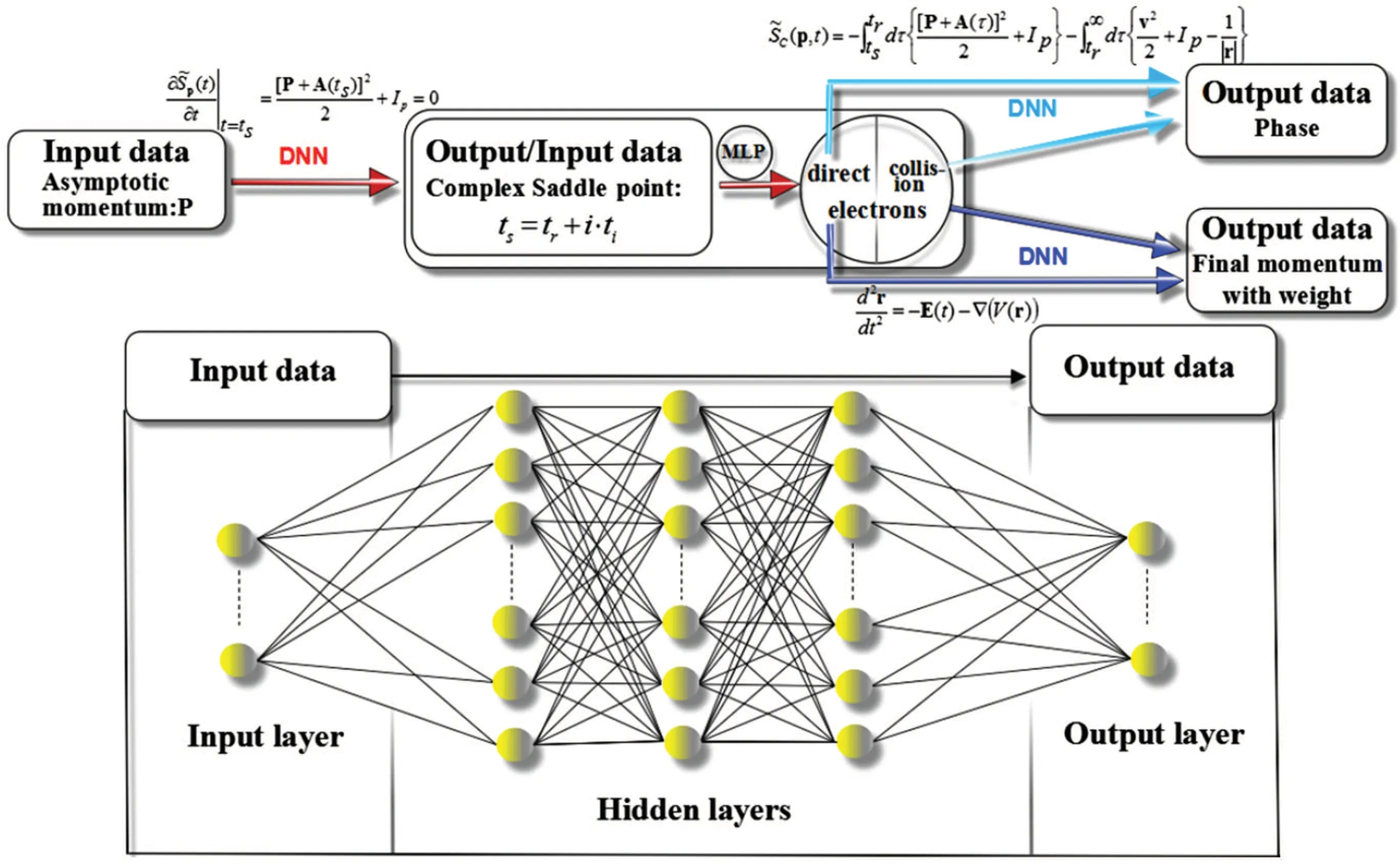
Fig.12. Schematic illustrations of deep learning. Adapted from Ref.[119].
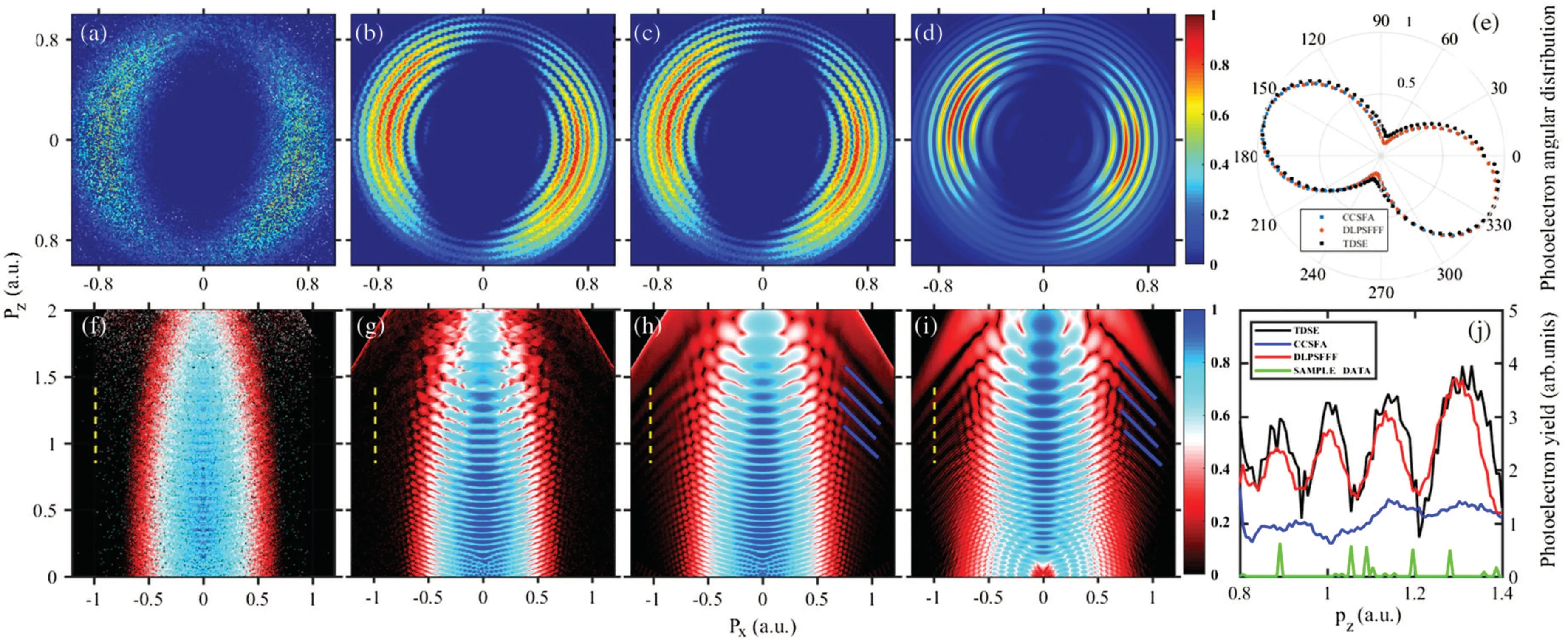
Fig.13. Comparison between the conventional simulations and the DLPSFFF predictions. The PMDs constructed with(a),(f)5×10⁵ sample training data,(b),(g)1×10⁸ trajectories simulated by the original CCSFA treatment,(c)1×10⁸,and(h)1×10¹⁰ data predicted by DLPSFFF,and(d),(i)quantum TDSE results.(e)The comparison of photoelectron angular distributions simulated by the CCSFA and TDSE with that predicted by DLPSFFF.(j)The photoelectron yield along Px0=-1 a.u. (the yellow dashed line)in panels(f)-(i). Adapted from Ref.[119].
Figure 13 shows the PMDs of hydrogen atom driven by an elliptically polarized laser pulses for different methods. Here, figure 13(a) showed the PMD constructed by the CCSFA approach with sampling training data of only 5×10⁵trajectories. The number of samples is too small to form a clear interference structure,while these number of trajectories are enough as sample training data to create a prediction tool in the DLPSFFF method. Figure 13(c)shows the final PMDs predicted by DLPSFFF method with the number of 1×10⁸trajectories. The PMDs showed typical ATI rings, which is in good agreement with the results obtained by CCSFA(Fig. 13(b)) and TDSE (Fig. 13(d)). In Fig. 13(e), the DLpredicted photoelectron angular distribution reproduces exactly the CCSFA result and the numerical solution of the TDSE.
The following example demonstrates another advantage of DFPSFFF, which is to help discover new phenomena in strong-field physics. The final PMDs obtained by CCSFA,DLPSFFF and TDSE methods are shown in Figs. 13(g)-13(i), respectively, it was found that the PMDs calculated by DLPSFFF and TDSE show an undetected oblique interference structure (denoted by blue solid lines) that is absent in the usual semiclassical CCSFA simulation,even with 108trajectories.This indicates that the DLPSFFF method has a significant contribution to the discovery of some new physical structures.This method will break the bottleneck of our current semiclassical method to calculate the time-consuming trajectories which provides a new method of optimization calculation.The DLPSFFF has a broad prospect and great potential to uncover the underlying physical mechanism.
6. Conclusion and outlook
In this paper, we review recent progress of semiclassical methods in trajectory analysis and information extraction in strong-field physics. Firstly, several mature semiclassical methods based on Feynman’s path-integral approach, such as GQTMC and CCSFA, are introduced. Compared with TDSE, the semiclassical methods provide clear physical images, and have natural advantages in extracting trajectory information and analyzing the physical mechanisms of certain interference structures. Then we introduce a spectral solution method(phase of phase)combined with GQTMC method to extract attosecond time delay in the process of photoelectric emission. Moreover, it had been used to discover different physical mechanisms that lead to attosecond time delay in above threshold ionization experiments, such as re-capture resonance scattering and Freeman resonance scattering mechanisms. Although semiclassical methods have been widely used in strong-field physics, there are still complex and massive data problems such as one by one traversal and force calculation. To tackle the problem about large calculation, the DLPSFFF method together with Rost’s[124]work open the study of strong-field physics with deep learning. This approach has a unique advantage in saving computational time and predicting new physical phenomena. It is expected to make the best use of semiclassical methods combined with advanced spectral resolution methods to analyze the ultrafast electron dynamics processes on attosecond scale,such as photoemission time reconstruction, identifying relevant contributions,etc.
Acknowledgements
Project supported by the National Natural Science Foundation of China (Grants Nos. 91950101, 12074240, and 12104285),Sino-German Mobility Programme(Grant No.M-0031), the High Level University Projects of the Guangdong Province, China (Mathematics, Shantou University), and the Open Fund of the State Key Laboratory of High Field Laser Physics(SIOM).
猜你喜欢
儿童故事画报·智力大王(2017年9期)2018-03-13
环球时报(2016-09-29)2016-09-29
时代英语·高二(2016年4期)2016-09-21
环球时报(2016-05-30)2016-05-30
英语学习·阳光英语(2013年2期)2013-07-04
民间故事选刊·上(2013年2期)2013-02-03

- Chinese Physics B的其它文章
- Measurements of the 107Ag neutron capture cross sections with pulse height weighting technique at the CSNS Back-n facility
- Measuring Loschmidt echo via Floquet engineering in superconducting circuits
- Electronic structure and spin-orbit coupling in ternary transition metal chalcogenides Cu2TlX2(X =Se,Te)
- Characterization of the N-polar GaN film grown on C-plane sapphire and misoriented C-plane sapphire substrates by MOCVD
- Quantum partial least squares regression algorithm for multiple correlation problem
- Optical scheme to demonstrate state-independent quantum contextuality