Speed Measurement Feasibility by Eddy Current Effect in the High-Speed MFL Testing

Zhaoting Liu,Jianbo Wu,★,Sha He, Xin Rao, Shiqiang Wang,Shen Wang and Wei Wei

1School of Mechanical Engineering, Sichuan University, Chengdu, 610065, China

2Safety Environment Quality Surveillance and Inspection Research Institute of CNPC Chuanqing Drilling& Exploration,Guanghan, 618300, China

3Chengdu Xionggu Oil & Gas Technology Co.,Ltd., Chengdu, 610000,China

4Chengdu Institute of Special Equipment Inspection and Testing,Chengdu, 610036, China

ABSTRACT It is known that eddy current effect has a great influence on magnetic flux leakage testing(MFL).Usually,contacttype encoder wheels are used to measure MFL testing speed to evaluate the effect and further compensate testing signals.This speed measurement method is complicated, and inevitable abrasion and occasional slippage will reduce the measurement accuracy.In order to solve this problem,based on eddy current effect due to the relative movement, a speed measurement method is proposed, which is contactless and simple.In the high-speed MFL testing,eddy current induced in the specimen will cause an obvious modification to the applied field.This modified field,which is measured by Hall sensor,can be utilized to reflect the moving speed.Firstly,the measurement principle is illustrated based on Faraday’s law.Then,dynamic finite element simulations are conducted to investigate the modified magnetic field distribution.Finally,laboratory experiments are performed to validate the feasibility of the proposed method.The results show that Bmz(r1) and Bmx(r2) have a linear relation with moving speed, which could be used as an alternative measurement parameter.

KEYWORDS Magnetic flux leakage testing (MFL); speed measurement; eddy current effect; modified magnetic field

1 Introduction

As an electromagnetic NDT(nondestructive testing)technology,magnetic flux leakage testing(MFL)is a powerful and highly efficient method and has been widely used for elongated ferromagnetic objects[1–6],such as pipelines[7–16]and rail tracks[17–23].In online or real-time MFL testing,permanent magnets are usually applied to magnetize the ferromagnetic specimen to saturation status [24–28].The magnetic flux lines are coupled into specimen using metal brushes or air coupling.If there are any anomalies or inclusions, the magnetic flux lines will leak outside the specimen in proximity of the anomalies and the sensor or sensor array will detect the leakage magnetic field.Specifically, according to Faraday’s law, due to the relative movement between inductive specimens and permanent magnets, apparent eddy current is generated in specimen under a high testing speed, namely eddy current effect.Consequently, this eddy current will generate magnetic field, change the magnetization status and influence MFL testing signals,including the amplitude and profile [29–34].In fact, the influence of eddy current effect on MEL method describes the influence of moving speed on the MFL testing.In order to evaluate eddy current effect and further compensate testing signals, several moves should be taken as follows: firstly, the influence rule of the scanning speed on MFL signals is obtained; and then, in the actual inspection the real-time moving speed is measured; finally, based on the measured speed and the influence rule, the sensitivity difference caused by scanning speed could be evaluated and further eliminated to obtain a consistent testing result[35].Besides, the scanning speed can be used for defect location.Hence, speed measurement is important in the scanning MFL testing.

In the traditional MFL scanning,the moving speed is usually measured by a contact-type way based on an encoder wheel, which bears against the specimen surface, generates pulse signals with its number in proportion to the scanning speed [36–43].However, there are measurement precision decreasing problems caused by the inevitable abrasion and occasional slippage of the encoder wheel, especially when the scanning inspection is performed at a high speed.In recent years, researchers have developed many contactless speed measurement methods.Gao et al.[44] developed a system using the CCD camera to measure the speed of the belt.However, this method not only requires expensive instruments, but also has high requirements on the appearance and shape of the specimen.Mirzaei et al.[45,46] came up with an interesting method that applies eddy currents to measure the speed of the train.But there is something cannot be neglected, that is, the device of this method is complex, and it requires additional electrical energy to power the coils.Using laser Doppler vibrometer to measure speed has the advantages of contactless and high accuracy [47].Nevertheless, this technique requires expensive instruments as well as complex analog and digital processing.The rotary laser scanning measurement systems is a simple and efficient method for measuring speed [48].Whereas, this system calculates the linear speed by measuring the angular speed.As a result, it is usually used to measure the speed of revolved bodies such as motors and disks, and it is not suitable for common MFL testing objects such as pipelines and rail tracks.Moreover, optical sensors are widely used for speed measurements [49,50], but they are not suitable for the MFL testing because of the obvious sensitivity to dirt and dust [46].Thus, a simple and contactless speed measurement method is in great need in the MFL detection.

According to Faraday’s law,when a conductive object moves in an external magnetic field,eddy current will be generated in the object.Based on this effect, in the scanning MFL inspection, relative movement between the magnetizer and specimen will produce eddy currents in the specimen and further cause a modification to the applied field.This modified field, of course, could be utilized to reflect the moving speed.Thus,a speed measurement method based on eddy current effect is proposed.

In this paper, the basic principle of the speed measurement is illustrated in Section 2 using a simple model based on Faraday’s law of electromagnetic induction.In Section 3, numerical simulations are conducted to investigate the distributions of the modified magnetic field.In Section 4, the speed measurement prototype is designed and developed, and then laboratory experiments are performed to preliminarily verify the feasibility of the novel method.Section 5 gives the conclusion.

2 Theoretical Model

The principle of MFL testing for ferromagnetic materials(e.g.,pipeline and rail tracks)is schematically illustrated in Fig.1, which shows a cross-section of the specimen, magnetizer and magnetic sensors.Two permanent magnets with opposite directions are mounted on a ferrite core.The use of ferrite core decreases magnetic resistance in the magnetic circuit and enhances the magnetic flux intensity in the specimen.Magnetic flux flows through the air gap, specimen wall and the ferrite core.If there are any anomalies or inclusions, the magnetic flux lines will leak outside the specimen in proximity of the anomalies.The magnetic sensor S1will detect the leakage magnetic field, which includes information of corrosions,cracks,etc.On the other hand,according to Faraday’s law,due to the relative movement between the magnet and the inductive specimen,eddy current is induced in the specimen around magnet poles.The eddy current will also generate magnetic field and further causes a modification to the applied field.This modified field can be measured by Hall sensors arranged at the P1and P2near the magnet poles, where the greatest modified magnetic field will be generated by eddy current.This modified magnetic field is utilized in the new speed measurement method.Compared to the traditional contact-type method by encoder wheel, the proposed method is contactless.Besides, the proposed method is simple and achievable,which changes nothing to the MFL apparatus except adding Hall sensors near the magnet poles.

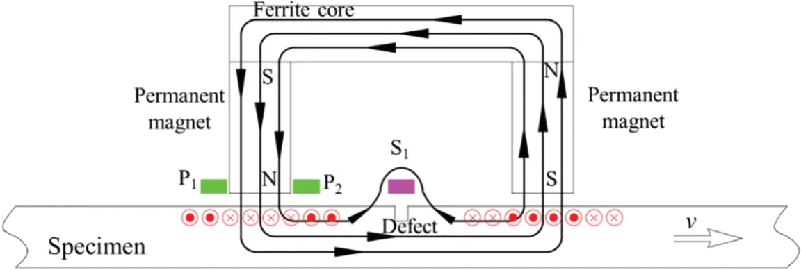
Figure 1: The speed measuring principle by the MFL device

In scanning MFL application,magnetizer moves along a conductive elongated object,such as pipelines and rail tracks.Here,theoretical model is approximated by a moving conductive plate and a fixed permanent magnet,as schematically illustrated in Fig.2.A permanent magnet,generating a constant external magnetic field Bex,is arranged above the conductive plate.According to Faraday’s law of electromagnetic induction,when the conductive plate moves in the Bexwith the speed of v,eddy current j1and j2will be induced in the object [51].Then, the eddy current will generate a magnetic field Binand cause a modification to the Bex.Thereafter, the modified magnetic field is measured by Hall sensors at the points P1and P2locating behind and in front of the permanent magnet along the moving direction.

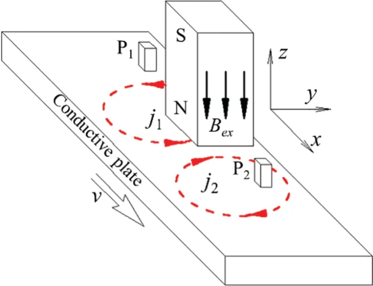
Figure 2: The principle of the speed measurement based on eddy current effect

As indicated in Fig.3,the relative movement between the permanent magnet and the conductive plate induces eddy currents that are governed by Ohm’s law for moving electrically conducting materials which has the form[52]

where, j(r),E(r),v(r)and B(r)denote the density of the eddy current,the electric field,the moving speed and the total magnetic field at the generic point r in the plate,respectively;σ denotes the conductivity of the plate.In Eq.(1),the term E(r)is the applied electric field,and the term v(r)×B(r)is the magnetization current term.

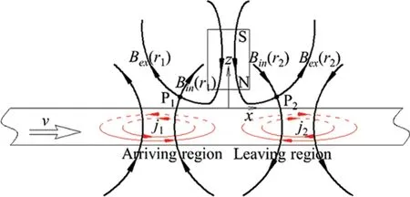
Figure 3: The distributions of the eddy current and the Bin at a low moving speed

Moreover,since there is no source or sink of electric currents in the plate,the electric field is zero.Then

The total magnetic field B(r) consists of the external magnetic field Bexgenerated by the permanent magnet and the induced magnetic field Bingenerated by the eddy current.Then

Eq.(3)indicates the scanning motion between the magnets and the specimen generates eddy current and then a Bin,which in turn influences eddy current distribution itself.

Applying Biot-Savart law,the magnetic field Binat the generic point r in the plate,is given by[53]

At measuring points P1and P2, the measured magnetic fields Bm(r1) and Bm(r2) captured by the Hall sensors are expressed as follows:

Based on Eq.(4),we can get

When the conductive plate moves at a low speed,the weak induced magnetic field Binin the plate can be neglected.Then, the Eq.(3) can be expressed as follows:

In Eq.(9), the magnetic flux density B can be calculated by multiplying the permeability μ by the magnetic field intensity H.In the theoretical analysis here, the permeability μ is assumed to be a constant.Then, the integral Eqs.(7)–(8) can be cast into a linear inverse problem for the determination of the speed from measured magnetic fields.

Figs.3 and 4 illustrate the distributions of the eddy current in the ferromagnetic object and the distributions of the magnetic fields in the air at low and high moving speed.Several black curves are drawn to represent the magnetic fields in the air, and several red curves are used to represent the eddy current fields in the ferromagnetic object.As schematically depicted in Fig.3, the external magnetic field Bex, generated by the permanent magnet, has a symmetrical distribution along z axis.Along the moving direction, the conductive plate can be divided into the arriving region and the leaving region, i.e., the region in the -x area and the region in +x area.Based on Eq.(9), the eddy current j1and j2in the arriving and leaving regions are distributed symmetrically along z axis and flow counter-clockwise and clockwise,respectively.

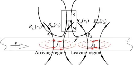
Figure 4: The distributions of the eddy current and the Bin at a high moving speed

However, when the moving speed increases to a high level, the eddy current will induce a strong magnetic field Binand then change the distribution of eddy current itself, i.e., self-inductance effect [30].The eddy current will not be immediately generated when the plate is moving below the permanent magnet.Consequently, with the moving speed increasing into a high level, the eddy current will be not symmetrical along the z axis and gradually moves to the leaving region,as depicted in Fig.4.

At the measuring points P1and P2,the measured magnetic field Bm,the external magnetic field Bexand induced magnetic field Bincan all be divided up into x components and z components.Based on Eqs.(5)–(6)we can get

where,Bmx(r1),Bmx(r2),Bmz(r1)and Bmz(r2)denote the x and z components of the measured magnetic fields at the points P1and P2,respectively;Bexx(r1),Bexx(r2),Bexz(r1)and Bexz(r2)denote the x and z components of the external magnetic field generated by the permanent magnet at the points P1and P2, respectively; Binx(r1),Binx(r2), Binz(r1) and Binz(r2) denote the x and z components of the induced magnetic field caused by the eddy current at the points P1and P2,respectively.

As illustrated in Fig.3, at low moving speed, the Binx(r1) and Binx(r2) both points in the positive xdirection; in contrast, the Binz(r1) points in the positive z-direction while the Binz(r2) points in the negative z-direction.With the moving speed increasing to a high level, since the eddy current j1and j2gradually move into the leaving region, Binx(r1) at the point P1firstly points in the positive x-direction at the low speed, and then points in the negative x-direction at the high speed, as displayed in Fig.4, respectively.As a result, based on Eqs.(10)–(13), the value of Bmx(r1) firstly increases and then decreases, while the other three components, i.e., Bmz(r1), Bmx(r2) and Bmz(r2), keep the same change trend during the increase of the moving speed.

3 Simulation Analysis

To investigate the distributions of eddy current and the modified magnetic fields,dynamic finite element modeling and simulation procedures are implemented in 2D by the commercial electromagnetic simulation software MAXWELL.The simulation model for speed measurement in a relative linear motion is built,as shown in Fig.5.The U-shaped magnet consists of two permanent magnets(Width:10.00 mm;Height:20.00 mm; Material: NdFe35) and a magnet yoke (Width: 50.00 mm; Thickness: 10.00 mm; Materials:steel_1008).The U-shaped magnet is arranged above a steel plate (Width: 2000.00 mm; Thickness:10.00 mm; Materials: steel_1008) with a liftoff value of 2.00 mm.The steel plate moves from the left side to the right.In actual MFL testing and past researches, the inspection apparatus scans the objects with speeds from 0.1 to 20 m/s [22,54–57].As a result, in the simulation, the U-shaped magnet remains stationary and steel plate moves at different speeds of 0.1, 1.0 to 20.0 m/s with step of 1 m/s.The distance of the two measuring points P1and P2is 15.00 mm.When the center of the plate arrives at the magnet, the x and z components of the magnetic field at the points P1and P2are simulated.And in addition to this, the eddy current distributions in the steel plate are observed and recorded when the speed is 0.1,1, 10 and 20 m/s, as shown in Figs.6–9.

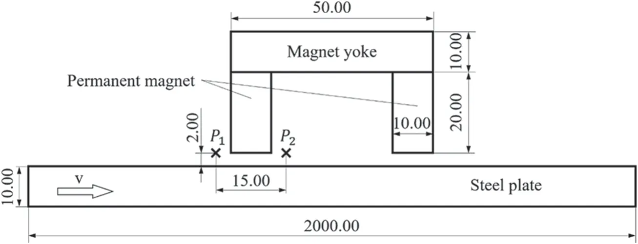
Figure 5: Simulation model for speed measurement based on eddy current effect(Unit: mm)

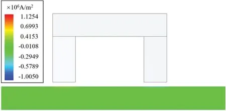
Figure 6: The eddy current distribution at the speed of 0.1 m/s

Figure 7: The eddy current distribution at the speed of 1.0 m/s

Figure 8: The eddy current distribution at the speed of 10.0 m/s

Figure 9: The eddy current distribution at the speed of 20.0 m/s

Figs.6 and 7 show the eddy current distributions in the steel plate at moving speed of 0.1 and 1.0 m/s,respectively.Fig.6 illustrates that there is almost no eddy current in the steel plate when the U-shaped magnet moves relative to the steel plate at ultra-low speed.Besides, Fig.7 shows that the eddy current has an approximately symmetrical distribution along z axis of each permanent magnet at low speed, matching well with the results of theoretical analysis,as displayed in Fig.3.

Figs.8 and 9 show the eddy current distributions in the steel plate at moving speed of 10.0 and 20.0 m/s,respectively.It can be seen that the eddy current moves into the leaving region and shows an asymmetrical distribution along z axis of each permanent magnet at high speed, which agrees well with the theoretical results, as depicted in Fig.4.

In order to obtain the accurate relationship between the measured magnetic field and the moving speed,the x and z components of the magnetic field at the points P1and P2are calculated and recorded.The trends of each component of the magnetic field are plotted and linearly fitted,as displayed in Fig.10.It can be seen that Bmx(r1)decreases nonlinearly and Bmz(r2)increases nonlinearly with the moving speed increasing.According to the results of the linear fit, it is worth noting that Bmz(r1) and Bmx(r2) both decrease linearly during the whole increase of the moving speed.Therefore, both Bmz(r1) and Bmx(r2) could be used as the ideal evaluation parameter.

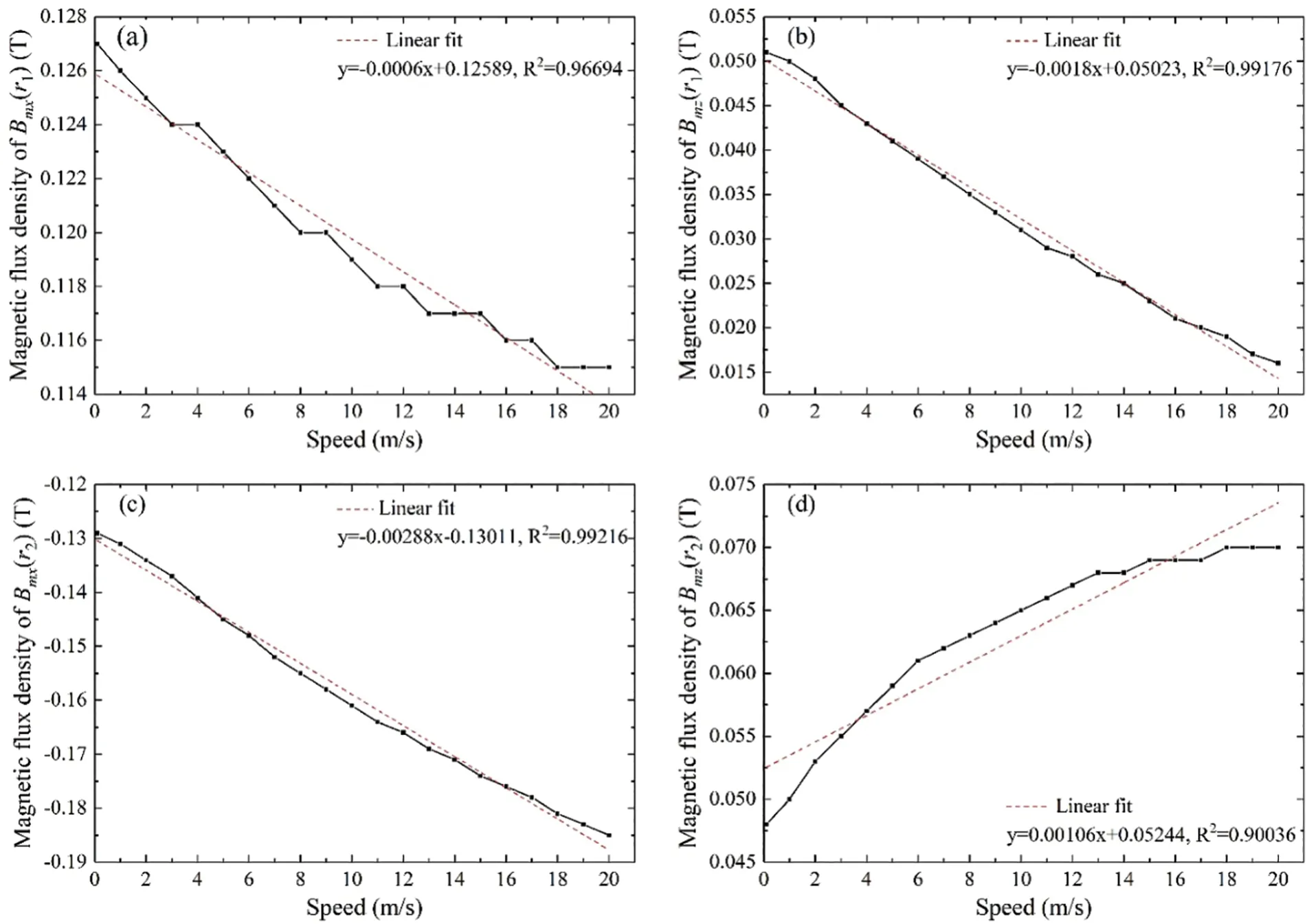
Figure 10: The simulation results of magnetic flux density at different moving speeds.(a) Bmx(r1);(b)Bmz(r1); (c) Bmx(r2);(d)Bmz(r2)

4 Experiment Validation

According to the speed measurement principle displayed in Fig.2 and the simulation model shown in Fig.5, a speed measurement prototype is designed and developed, as pictured in Fig.11.The prototype consists of a U-shaped magnet and a printed circuit board (PCB).The U-shaped magnet is composed of two permanent magnets (Length: 20.00 mm; Width: 10.00 mm; Height: 20.00 mm; Material: NdFe35)and a magnet yoke (Length: 20.00 mm; Width: 50.00 mm; Thickness: 10.00 mm; Materials: Steel 45).Four Hall sensors (Manufacturer: ALLEGRO; Type: A1302) are soldered on the PCB.And the four Hall sensors are placed at points P1and P2in Fig.11.Specifically, the four Hall sensors are divided into two groups to measure the x and z components of the magnetic field at the points P1and P2.The two-group Hall sensors are properly arranged with a distance of 15.00 mm to avoid being saturated by the permanent magnet.The use of PCB ensures the accuracy of the positions of points P1and P2.

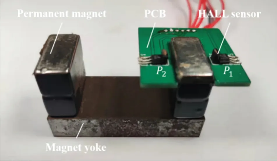
Figure 11: The prototype designed based on the simulation model

Then,the apparatus for the experiment was set up,as displayed in Fig.12.The device of the experiment is made up of a prototype, a battery pack, a voltage conversion module, an oscilloscope (Manufacturer:Tektronix; Type: MDO4034C), a three-phase synchronous motor and a steel disk (Diameter:1200.00 mm; Thickness: 20.00 mm; Materials: Steel 20).The prototype is shown in Fig.11.The battery pack and voltage conversion module together provide pure 5-volt power to the Hall sensors soldered on the prototype.This power supply is extremely precise.According to the ripple test results, the peak to peak of its ripple is only 5 mV.In other words, its accuracy is as high as 0.1%.The oscilloscope has four channels, which are connected to the output pins of the four Hall sensors on the prototype to measure their output voltages.The three-phase synchronous motor and steel disk constitute the motion system of the experimental device.The three-phase synchronous motor controlled by an inverter drives the steel disk to rotate at different speeds.

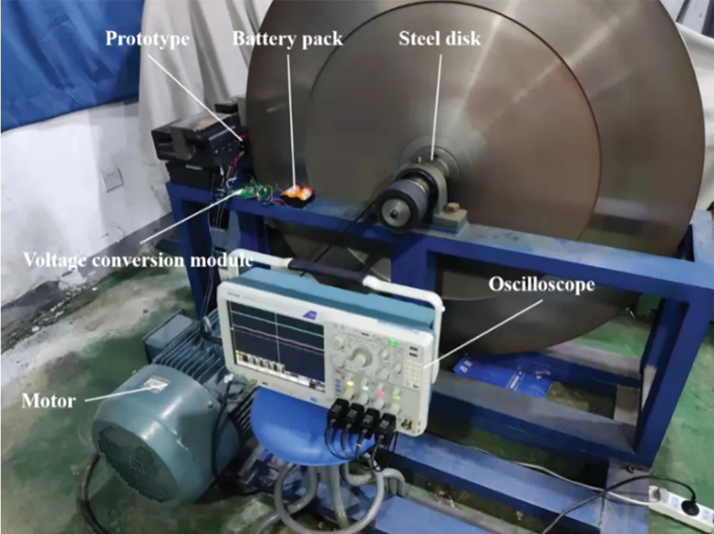
Figure 12: The device of the speed measurement experiment

In addition to the basic information on the experimental device above, some details about the experimental device must be elaborated.The prototype is fixed on the fixture made of polylactic acid(PLA), which does not affect the magnetic field distribution of the prototype.In order to ensure the consistency of the experimental device and the simulation model, the permanent magnet with the PCB is placed upward, and the steel disk moves counter-clockwise, as shown in Fig.13.Furthermore, the prototype is placed at the edge of the disk with a liftoff value of 2 mm.An aluminum sheet with a thickness of 2 mm is employed to ensure the accuracy of this liftoff value.

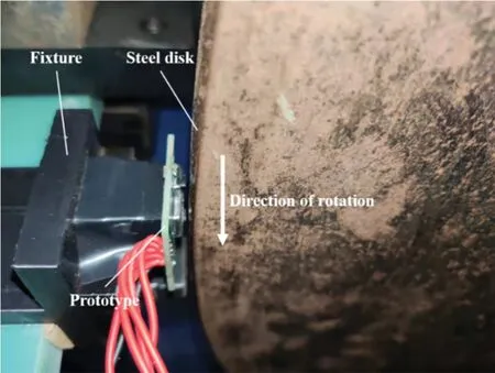
Figure 13: The partial enlarged view of the prototype and the steel disk

After the experimental device is built, a sequence of laboratory experiments is performed to preliminarily investigate the feasibility of the proposed method.The moving speed of the steel disk is controlled by adjusting the frequency of the motor.Based on the previous measurements using the encoder wheel, the angular speed of the steel disk varies linearly with the frequency.The relative linear moving speed between the prototype and the disk can be calculated by multiplying the radius and the angular velocity.In the experiment, the frequency of the motor is increased from 0.1 to 5.7 Hz with step of 0.3 Hz.Correspondingly, the moving speed of the circumference of the steel disk changes from 0.99 to 20.01 m/s.When the disk rotates in a stable revolution speed, the four components of the magnetic field are captured by the four Hall sensors.In the experiment, the oscilloscope is employed to measure the output voltage values of the four Hall sensors.At a steady speed, a huge quantity of output values is collected from each Hall sensor.These values are averaged with the help of the mathematical software MATLAB.During the experiment, it is very important to measure and average a large number of output voltage values of each Hall sensor.This mathematical treatment will tremendously increase the accuracy of the measured speed.Nevertheless, this treatment will bring some shortcomings.For instance, an excessive number of samples will result in an increase in the response time.Therefore, in practical applications,the choice of sample size is crucial.

In this experiment,100 k voltage values are collected and averaged.After data processing,the average signal values of each Hall sensor are obtained at each measured speed.The average signal values of the four components of the magnetic field at different speeds are displayed in Fig.14.And the magnetic field consists of the external magnetic field generated by the permanent magnet and the induced magnetic field caused by the eddy current.Comparing Figs.10 and 14,it is obvious that the experimental results and the simulation results are in very good agreement.To be more specific, with the moving speed increasing from 0.99 to 20.01 m/s, it can be seen that the average signal values of the four components have the same change trend with the simulation results as shown in Fig.10.Bmx(r1) decreases nonlinearly, and Bmz(r2) increases nonlinearly.In particular, during the whole increase of the speed,the Bmz(r1) and Bmx(r2) all show a linear increase with respect to the moving speed, as shown in Figs.14b and 14c.Hence, in the practical application,the Bmz(r1)and Bmx(r2)could be chosen as the ideal evaluation parameter.

Besides,the linear fitting equations of the data collected by each sensor and the R-squared(R2)of the fitting curves are also shown in Fig.14.In Figs.14b and 14c, the R2of the fitting plots are 0.99497 and 0.99505, respectively.Hence, the average signal value of Bmz(r1) and Bmx(r2) all have very good linearity with respect to the speed.To further verify that the proposed method has high accuracy, the average signal value of Bmz(r1) is taken as the signal feature for speed measurement.At a known speed, the average signal value of Bmz(r1) is obtained and put into the linear fitting equations in Fig.14b to calculate the speed.And the results of speed measured by the average signal value of Bmz(r1)are shown in Table 1.The average error rate calculated from the data in Table 1 is only 2.24%.Obviously, high accuracy can be obtained by using the method proposed in this paper.

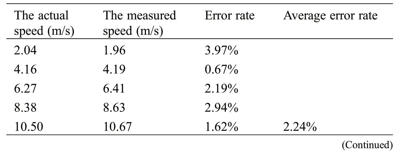
Table 1: The speed measurement error

Permanent magnet with different liftoff distances from the specimen surface generates a different external magnetic field distribution above the specimen.Based on Eq.(3), the changed external magnetic will influence the eddy current and further produce a different signal response in the measurement sensor.In order to investigate the liftoff effect in the speed measurement, the measurement sensor is placed with different liftoff distances varying from 1.0 to 3.0 mm with a step of 0.2 mm.In the experiment, the steel plate is driven to rotate at a fixed moving speed of 10 m/s.Fig.15 shows the measured average signal values of Bmx(r2) at different liftoff distances.It can be seen that with the liftoff distance increasing, the measured average signal value shows a sharply decreasing trend.Thus, on the one hand, in order to obtain a high sensitivity, the speed sensor should be placed close to the inspected objects if possible.On the other hand, in the practical application, the speed sensor should be arranged at a fixed liftoff distance to avoid the sensitivity difference caused by a varied liftoff distance.

Figure 15: The measured average signal value at different liftoff distances with moving speed of 10 m/s

5 Conclusion

In this paper,a contactless speed measuring method based on eddy current is proposed in the scanning MFL testing.Different from the traditional contact method by encoder wheels, the proposed method is a contactless way, which creatively utilizes the relative movement between the specimen and magnets to induce eddy current for speed measurement.The proposed method could be taken as a supplement.The combination of the traditional contact method and the proposed contactless one could greatly improve the measurement accuracy, which will be investigated in the future works.Additionally, the proposed method is simple and achievable,which changes nothing to the MFL apparatus expect adding Hall sensors near the magnet poles.It can be concluded that:

(1) At low moving speeds,owing to the weak induced magnetic field,the eddy current j1and j2in the arriving and leaving regions have a symmetrical distribution along z axis of each permanent magnet.In contrast,at high moving speeds,the eddy current distribution will be altered by self-inductance effect and move into the leaving region.Simulations and experiments show that the Bmz(r1) and Bmx(r2) show a linear decrease with respect to the moving speeds from 0.1 to 20.0 m/s, which could be used as the ideal evaluation parameter.

(2) The measured average signal value of Bmx(r2) shows a sharply decreasing trend with the liftoff distance increasing.Thus, on the one hand, in order to obtain a high sensitivity, the speed sensor should be placed close to the inspected objects if possible.On the other hand, in practical application, the speed sensor should be arranged at a fixed liftoff distance to avoid the sensitivity difference caused by a varied liftoff distance.

Acknowledgement:Funding from the National Natural Science Foundation of China and the Sichuan Science and Technology Program is gratefully acknowledged.

Funding Statement:This work is supported in part by the National Natural Science Foundation of China(Grant No.92060114), in part by the Sichuan Science and Technology Program (Nos.2022YFS0524 and 2022YFG0044).

Author Contributions:The authors confirm contribution to the paper as follows: study conception and design: Jianbo Wu, Zhaoting Liu; data collection: Zhaoting Liu, Sha He, Shiqiang Wang; analysis and interpretation of results: Xin Rao, Shen Wang; draft manuscript preparation: Zhaoting Liu, Wei Wei.All authors reviewed the results and approved the final version of the manuscript.

Conflicts of Interest:The authors declare that they have no conflicts of interest to report regarding the present study.