
A synchronous scanning measurement method for resistive sensor arrays based on Hilbert-Huang transform
2024-01-08 09:10TONGZhixueFENGWenjunCAOHengyuanCHANGShengZHANGXuefeng
TONG Zhixue,FENG Wenjun,CAO Hengyuan,CHANG Sheng,ZHANG Xuefeng
(School of Mechanical and Electrical Engineering,Xi’an University of Architecture and Technology,Xi’an 710055,China)
Abstract:The current spectrum analysis method cannot perform synchronous scanning on the resistance sensor array.The Hilbert-Huang transform (HHT) with improved empirical mode decomposition is innovatively applied for the spectrum analysis of the response signal of the resistive array.First,the endpoint effects in the processing of empirical mode decomposition (EMD) are introduced.Aiming at the endpoint effect phenomenon in processing of EMD,the extension method which is appropriate to deal with the response signal of the resistive array is obtained by comparing three different kinds of extension methods.Then the improved algorithm is used for the spectrum analysis of the response signal of the resistive array.And the relations of all units’ resistance and time,frequency and amplitude are obtained.In this way,all elements in the whole array can be accessed and measured.Finally,the effectiveness of the improved HHT is verified by simulation experiments.The results show that the improved algorithm can obtain the precise time-frequency distribution of all the elements in the array,which can promote the application of measurement method with AC power source in the field of resistive sensor array measurement.
Key words:Hilbert-Huang transform (HHT); resistive sensor array; AC measurement; endpoint effect; frequency spectrum analysis
0 Introduction
The resistive sensor can convert external physical excitation into an electrical resistance signal output.As a type of device,it is widely used in the engineering field.However,a single resistive sensor unit cannot complete the measurement task in certain application scenarios such as pressure distribution measurement of plane or surface,and a reasonable arrangement of multiple sensor units in array form can achieve desired functions.Due to the high resolution and ease of implementation,resistive sensor arrays are widely used in many fields such as status detection,fault diagnosis,biomedicine,and intelligent robots,and so on[1-3].
If the signal of each sensor unit in the resistive sensor array needs to be derived through an independent wire,then the number of wires for a resistive array sensor withMrows andNcolumns becomes 2MN.It will increase the complexity of the structure undoubtedly.By connecting one end of each sensor unit to the row electrode and the other end to the column electrode to form a sharing row and column electrodes structure,the number of wires will be greatly reduced toM+N.This advantage is particularly significant in a large number of sensor arrays.However,crosstalk is introduced by the structure,which increases the difficulty of reading the sensor unit and reduces the measurement accuracy[4-5].Many solutions have been proposed to eliminate crosstalk by installing additional transistors on the row or column interface[6-7],and gating of the sensor unit by controlling the on and off of the transistor can read every units individually.Voltage feedback method[8-9]and zero potential method[10-12]are also widely used to suppress crosstalk among units.The mechanism of the two methods is to form an equipotential area on both sides of non-target sensor units to eliminate the influence of crosstalk on the measurement of target sensor unit.All of these methods adopt a DC power as the excitation signal.However,additional measurement deviations is introduced due to the non-ideality of used devices,and this inaccuracy will increase as the sensor array becomes larger[11-12].
In order to improve the measurement accuracy,Zheng Hu et al.proposed an AC measurement method[13-14].A series of single-sine-wave with different frequencies are utilized as excitation signals of each row to achieve non-interference among rows.This method does not require a multiplexer to complete the gating of the row electrodes,so it can effectively eliminate the measurement deviation caused by the on-resistance of the multiplexer.By employing the AC excitation signals,the effect of DC bias voltage of the operational amplifier can also be suppressed.In order to measure the resistance of the sensor units located at nodes with different rows and the same column of electrodes,it is necessary to extract multiple sinusoidal signals (multi-sine-wave) of different frequencies on the column electrodes.Fast Fourier transform (FFT) is used to process multi-sine-wave.In practical applications,the resistance of the resistive sensor changes at any time and is a non-stationary signal.However,the Fourier transform is based on the assumption of the stationarity of the signal.Then the analysis results only reflect information in frequency domain without the time domain characteristics[15].
In order to obtain the time-frequency characteristics of the resistance value of each sensor unit of the resistive sensor array,an improved empirical mode decomposition (EMD) method and Hilbert transform are used to process the response signal of the resistive sensor array.Then the resistance value of each sensor unit at different moments are achieved according to Hilbert spectrum analysis method.Finally,a resistive sensor array is used to illustrated the validity of the method.Results show that the improved spectrum analysis can quickly and accurately decompose the resistance value of each resistor at each moment.
1 AC excitation measurement method
1.1 Circuit principle
For the special structure of the resistive sensor array,as shown in Fig.1,single-sine-wave of different frequencies are used to drive each row separately.The single-sine-wave voltage of themth row isVAC,m.Its frequency isωm.The amplitude of AC voltage source isAm.The initial phase isφm,and its mathematical expression is
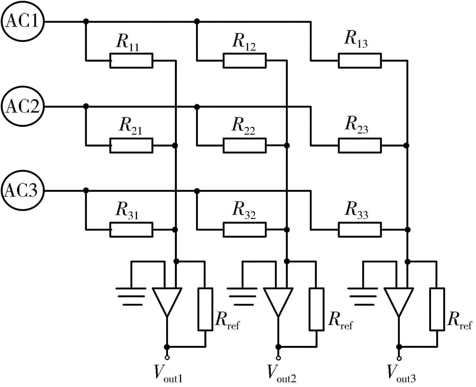
Fig.1 AC excitation resistive array sensor measurement circuit
VAC,m=Amsin(ωmt+φm).
(1)
The AC voltage sources of different frequencies are independent of each other in the frequency domain.All resistors in the same column together with their operational amplifiers form an AC voltage summing circuits.The current flowing through each resistor is a single-sine-wave with a specific frequency.Grounding the non-inverting input of the operational amplifier,the output signal of thenth column operational amplifier is a multi-sine-wave containingMindependent frequency components.The output signal can be expressed as
(2)
whereBmnis the maximum amplitude of the multi-sine-wave at the frequency pointωm.According to the principle of the AC voltage summing circuit,the resistance value of the sensor connected to themth row and thenth column can be calculated by
Rmn=Rref(Am/Bmn),
(3)
whereRrefis the feedback resistance;Amis the amplitude of AC voltage source,andBmnis the measured amplitude of the multi-sine-wave at the frequency pointωm.
In order to quantitatively compare the deviation of the measurement result from the true value,the measurement error is defined as
(4)
whereRmis the measurement result andRris the true value.
1.2 Theoretical analysis
The resistance of all the units in a resistive array with sharing row and column electrodes structure can be measured by applying AC excitation signals with different frequencies to each row and performing spectrum analysis for the responding signals from each column of the array,respectively.Taking an AC circuit as an example as shown in Fig.2(a),it consists of an AC voltage source and a resistorR.Suppose that the AC voltage source is

(a) Circuit model
VAC=Asin(ωt+φ).
(5)
According to the Ohm’s law,the instantaneous current of the resistor is
(6)
The direction of current has no effect on the resistance in AC circuit.As shown in the Fig.2(b),the current and voltage have the same transformation trend.In other words,the current and voltage have the same frequency and phase.
A 3×3 resistor array is taken as an example to analyze the resistance of the first column.The other columns are similar to the first column.The single-sine-wave of different frequencies are used to drive each row separately.And each row is composed of an AC voltage source and three resistors.The resistance of the first column in the array is simplified as shown in Fig.3.
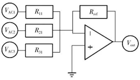
Fig.3 Simplified model of first column resistance in array
Each branch is equivalent to the three AC circuits in parallel.Since all branch currents are in phase,all single branch currents can be added together.Finally,it forms a negative feedback circuit with the operational amplifier,and the output signal of the operational amplifier is a multi-sine voltage containing three independent frequency components.The output signal can be written as
(7)
1.3 Circuit model
In order to compare the performance between HHT and FFT in spectrum analysis,a 3×3 resistive array is built by Multisim software for simulation,as shown in Fig.4.The operational amplifier on column is ADA4655,and the feedback resistance of each column is 2 kΩ.The power supply is ±16 V,and the reference voltage is 0 V.A sliding rheostat marked asR31is specified as the measurement targeted resistor to simulate the resistive sensor (at the intersection of the third row and first column).The resistance changes from 100 Ω to 1 000 Ω with the interval of 100 Ω,while other un-targeted resistances are set to 100 Ω.Each row of the array is excited by a single-sine-wave of the same amplitude (0.1 V) and phase (0°) with different frequencies.Finally,the output signal is collected to perform spectrum analysis.
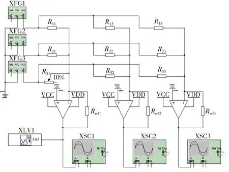
Fig.4 Resistive sensor array circuit model
2 Endpoint effect of HHT and its treatment method
2.1 Endpoint effect
HHT was proposed by Huang E and others mathematicians.It is a new signal time-frequency analysis method.This method is regarded as the most important discovery in the field of applied mathematics by National Aeronautics and Space Administration in recent years.HHT is mainly composed of EMD and Hilbert transform[16].Among them,EMD decomposition is the core of HHT transformation.The EMD method decomposes the complex signal function into the sum of finite intrinsic mode functions (IMFs) based on the local characteristic time scale of the signal itself.Then Hilbert transform is performed on each IMF component to obtain the amplitude and instantaneous frequency of each IMF component changing with time.Finally,the Hilbert time-frequency spectrum diagram of amplitude-frequency-time is obtained,and the amplitude transformation of each sensor unit at different times is obtained through the time-frequency spectrum diagram.
In EMD decomposition,the extrema of the signal is used as the interpolation point,and the cubic spline interpolation algorithm is used to construct the upper and lower envelopes,and then the mean value of the signal is obtained.This decomposition process is called screening.However,the endpoints of the signal are not the extrema ingeneral,the spline curve diverges at the endpoints of the data series.This divergence gradually spreads inward as the screening process continues,and it will make the IMF lose its physical meaning in some severe cases.This phenomenon is named as the endpoint effect[16-18].The endpoint effect is inevitable in the decomposition of EMD.Fig.5 shows the endpoint effect in the cubic spline interpolation algorithm process of a column electrode signal.It can be seen that there is a large amplitude change both at the left endpoint (0.2 s) and the right endpoint (0.3 s).This result suggests that the endpoint should be suppressed to acquire accurate measurement results.
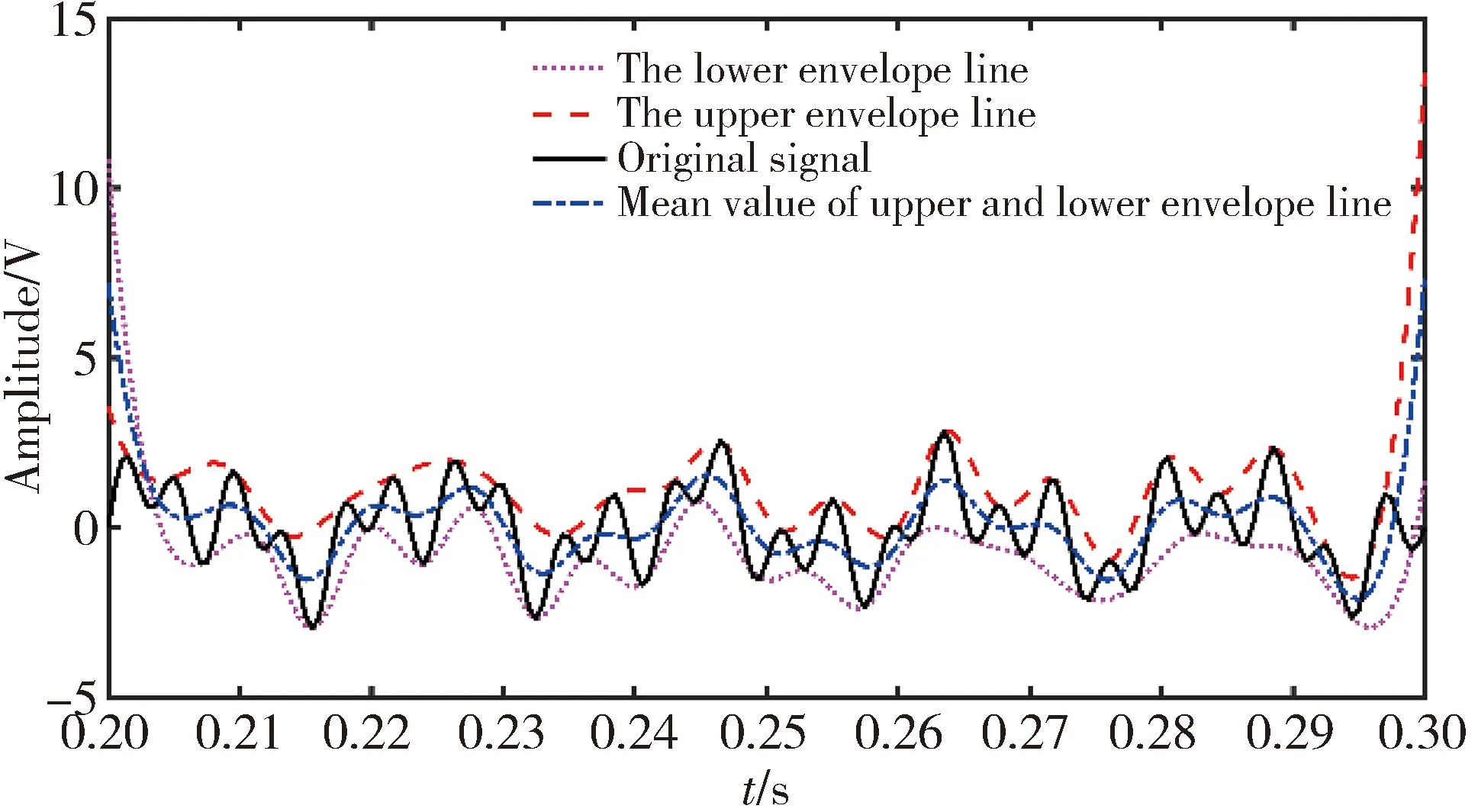
Fig.5 Endpoint flying wing phenomenon by cubic spline interpolation
There are two main ways to suppress the endpoint effect.One is to use other forms of spline function to fit the curve,but their interpolation performance may be worse than cubic spline.The other is the endpoint extending method,which is to find the appropriate extrema at both ends of the data sequence,so that the upper and lower envelopes of the signal fitting can envelop the entire signal.Among them,the endpoint extending method has been widely used.Currently,6 kinds of endpoint extending methods are commonly used.The neural network extending method[19],the waveform matching extending method[20]and the support vector machine extending method[21]have slow calculation speeds which do not meet the practical application requirements of the resistive sensor array.The extremal mirror image extending method[22],the boundary local characteristic scale extending method[23]and the polynomial fitting extending method[24]have good real-time performance,which can meet the practical application requirements of resistive sensor array.In fact,the suppression effect of the extending method is also related to the characteristics of the signal itself.To compare the three extending methods,the collected signal from the resistive array is numerically simulated and analyzed.
2.2 Endpoint effect evaluation index
Three evaluation indexes(i.e.,similarity coefficientρ,average relative error RMSE and operation time) are adopted to illustrate the advantages and disadvantages of three different EMD endpoint suppression methods.
1) After EMD decomposition,the similarity coefficientρbetween each component signal and the corresponding original signal is calculated according to Eq.(8).Due to the shape distortion of the signal envelope,the endpoint effect will be introduced,which makes the decomposition of each component inaccurate.By comparing the similarity between IMF components and original signal components after EMD decomposition,the suppression effect of each endpoint extending algorithm can be evaluated by
(8)
where cov() represents the covariance; σ() represents the variance; IMFirepresents theith modal component of the signal after EMD decomposition;xiis the corresponding component of the original signal.The greater theρvalue,the better the inhibition effect of endpoint effect.
2) Average relative error RMSE among IMF components obtained by EMD decomposition and corresponding components of original signal can be calculated by[25]
(9)
whereNrepresents the total number of signals;xiand IMFiare the same as Eq.(8).The smaller the σ,the better inhibition effect of endpoint effect.
3) The method takes the least time to suppress the endpoint effects to meet real-time requirements.
2.3 Simulation results
A multi-sine-wave is simulated by numerical simulation,where the sampling frequency is 3 200 Hz,the number of sampling points is 320,and the sampling time is 0.1 s.The expression is
y(t)=sin(100πt)+sin(230πt)+sin(480πt).
(10)
After EMD decomposition of the simulation signal,three IMF components sorted as high frequency components,intermediate frequency components and low frequency components are shown in Fig.6.By comparing IMF components with ideal components without endpoint effect,it can be seen that all of three methods can suppress endpoint effect to some extent.
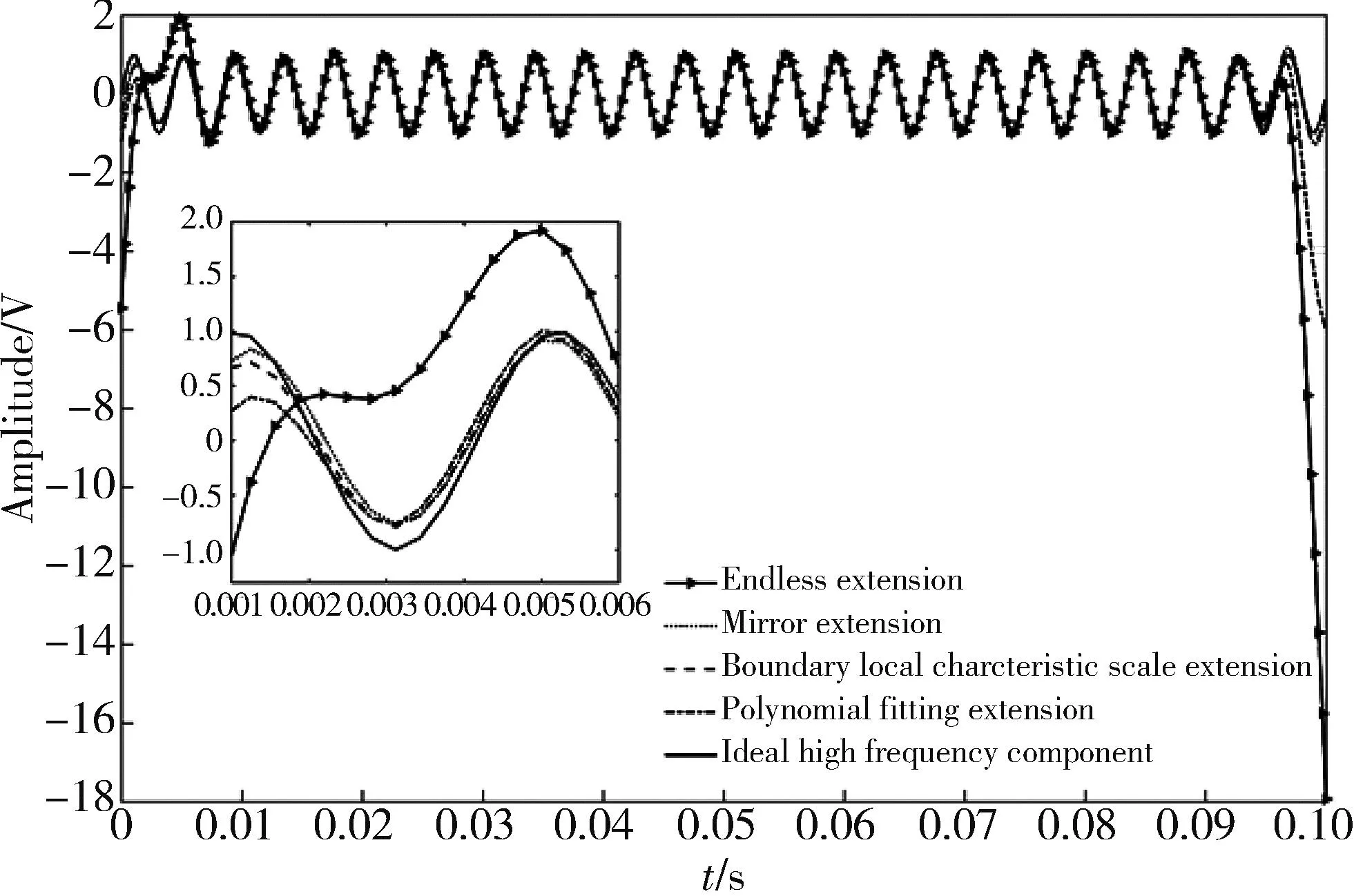
(a) Comparison for high frequency components
It can be seen that the frequency is lower,and the end-point flying wing phenomenon is worse.It shows that the error at the endpoint will gradually accumulate with the screening process.And as the final screening out of the low frequency component,the error is also the largest.After endpoint processing,it is found that the endpoint flying wing phenomenon of low-frequency components has been significantly improved,indicating that the three continuation methods have suppressed the endpoint effect of EMD decomposition.The extremal mirror image extending method and the boundary local characteristic scale extending method have better inhibitory effect on polynomial fitting method,but the difference between the extremal mirror image extending method and the boundary local characteristic scale extending method is not obvious.It is necessary to further analyze the endpoint evaluation index.The performance of three improved EMD decomposition methods is listed in Table 1.
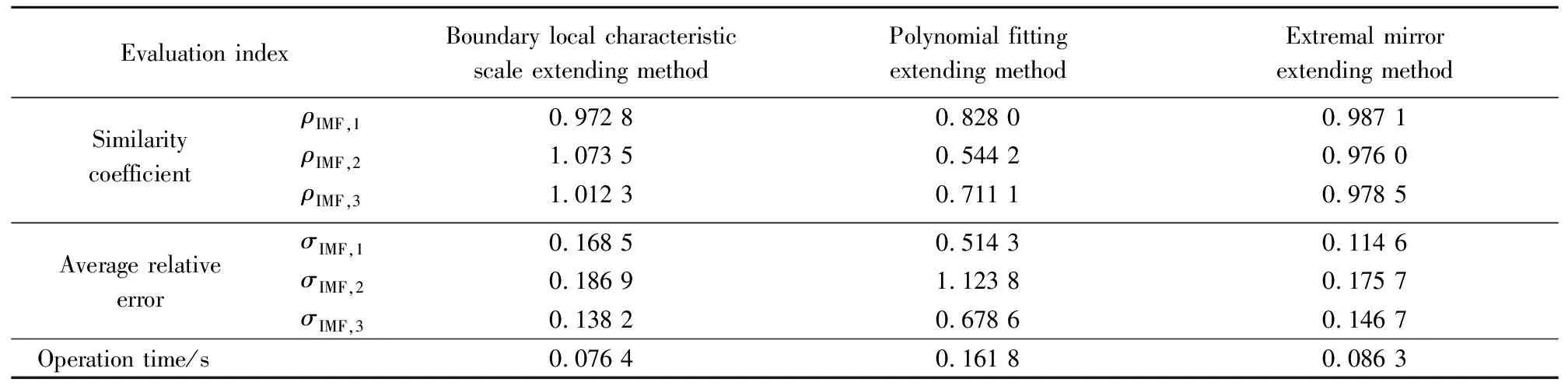
Table 1 Performance evaluation of endpoint suppression method
It can be obtained that the similarity coefficient of boundary local characteristic scale extending method is the largest,and its average relative error is close to the extremal mirror image extending method.The polynomial fitting method has the smallest similarity coefficient,the largest average relative error and the lowest decomposition accuracy.As to the operation time,it can be seen that the operation time of the boundary local characteristic scale extending method is the shortest.Therefore,the boundary local characteristic scale extending method is designated according to the characteristics of the signal.
3 Experiment
The acquisition signal of the AC-excited resistive array is a multi-sine-wave which is a superimposed signal of a plurality of sinusoidal signals.And the HHT method is suitable for processing multi-component signals.Its advantage is that it is not limited by the number of rows and columns of the resistor array,and the method is not affected by the difference in resistance values.Therefore,the resistance changes of the resistive array in the steady state and dynamic states are analyzed through simulation experiments.
3.1 Simulation analysis of steady-state resistance
The targeted resistive sensorR31and other un-targeted resistive sensor are set to be 100 Ω.The frequency of each row is set to 50 Hz (the first row),300 Hz (the second row) and 1 800 Hz (the third row),respectively.The sampling frequency is 30 kHz,and the sampling time is 0.05 s.The collected data are processed by FFT and the improved HHT method,respectively.Fig.7 shows the EMD decomposition diagram of the collected data.

Fig.7 Acquisition signal and its IMF components
The third-order IMF components are obtained after the endpoint effect is eliminated by the boundary local characteristic scale extending method,which is arranged in descending order of frequency.The Hilbert transform is performed for each order IMF component to obtain the corresponding instantaneous frequency and amplitude,and the consequent Hilbert Huang spectrum is shown in Fig.8.It can be seen that the amplitude remains unchanged in the sampling time at a specific frequency.
Due to the unique advantages of the FFT algorithm in processing stationary signals,the FFT algorithm is selected to compare with the improved algorithm.The measurement results are shown in Table 2.The FFT algorithm has little difference with the improved algorithm in terms of frequency.However,the inproved algorithm can measure the target resistance accurately at each frequency,and the resistance measured by the FFT method is far from the target resistance.Therefore,the improved algorithm is better than the FFT algorithm.

Table 2 Steady-state resistance measurement results
3.2 Simulation analysis of dynamic resistance
In practical application,the resistance value of resistive sensor is time varying.In order to comply with reality,the first column of collected signals is still taken as an example in the simulation.R31is used as the targeted resistance,and the sliding rheostat is used to replace the dynamic resistance.The measurement range is from 100 Ω to 1 000 Ω,the measurement time is 1 s,and the resistance value increases by 100 Ω every 0.1 s.The frequency of each row is 50 Hz (the first row),300 Hz (the second row) and 1 800 Hz (the third row).The sampling frequency is 30 kHz.The collected signal of time-varying resistance and the IMF components of each order after EMD decomposition are shown in Fig.9.Among them,IMF1 is the amplitude change of the measured target resistanceR31,and it is found that the amplitude changes step by step,and the time of each change is roughly corresponding to the time of the change of the sliding resistor.
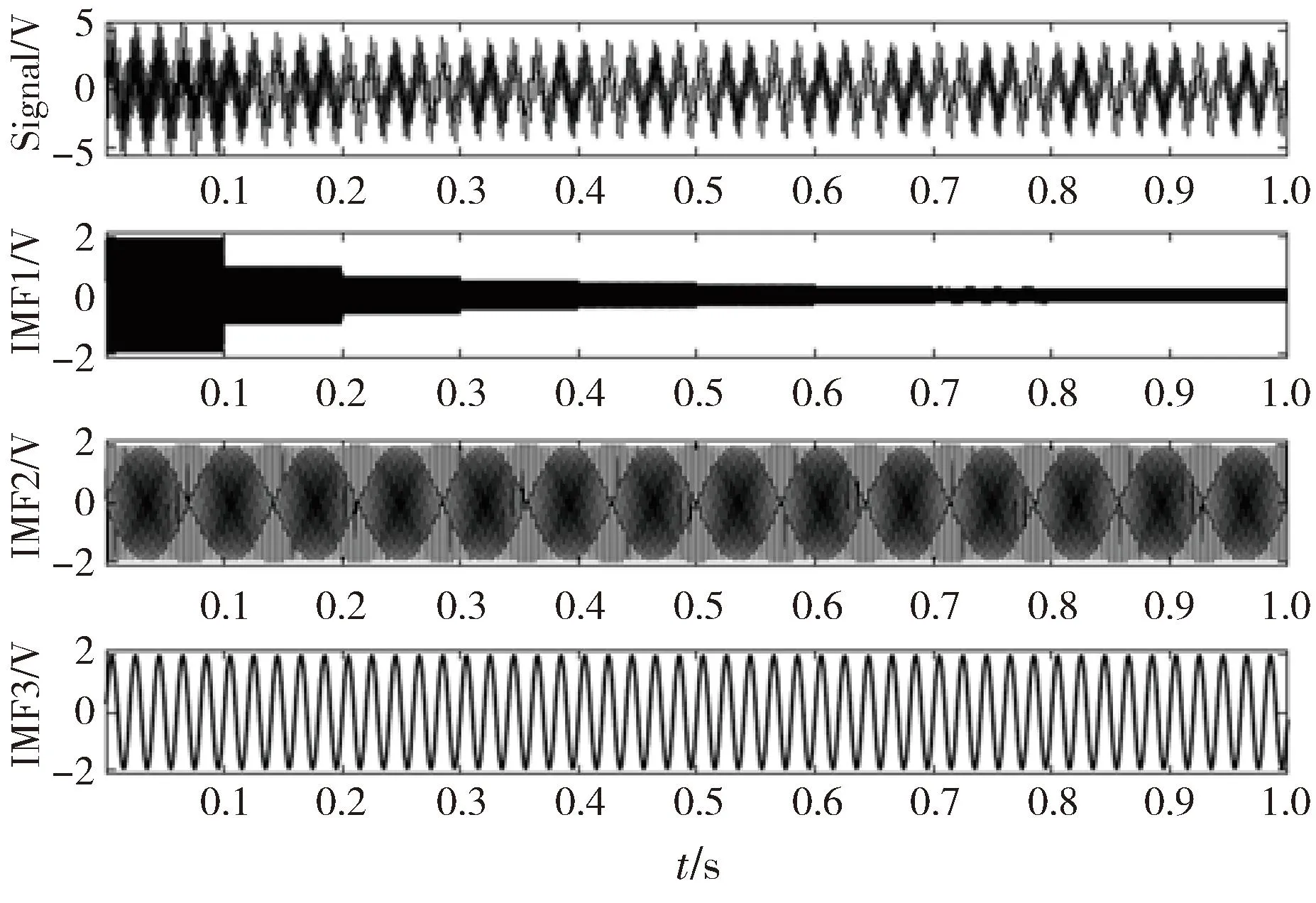
Fig.9 Collected signal of dynamic resistance and its IMF components
In order to understand the amplitude change of the target resistance more accurately,the Hilbert transform is performed on the IMF1 component to obtain the resistance amplitude change diagram as shown in Fig.10.
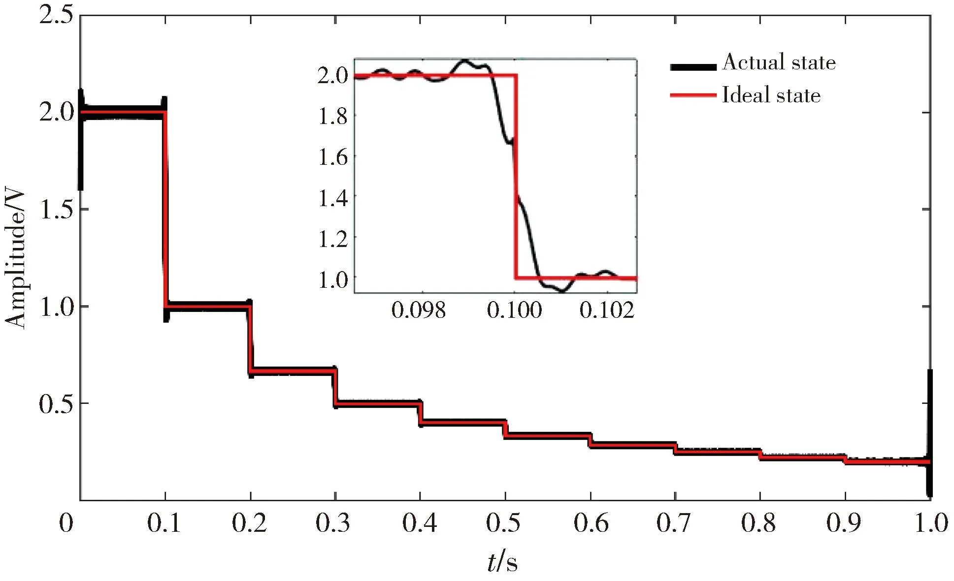
Fig.10 Changes in the amplitude of target resistance
It can be seen that the amplitude of the target resistance has a high accordance with the ideal state.Table 3 shows the measurement results of dynamic resistance.It can be seen that both the measured resistance value and the measured frequency have very small errors compared with the frequency and resistance value of the real signal.All of these results show that the improved method has good practical application prospects.
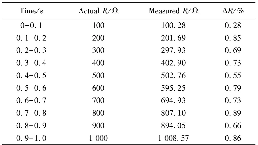
Table 3 Dynamic resistance measurement results
4 Conclusions
The HHT algorithm is used in the signal processing of the resistive array sensor based on the AC excited method,which overcomes the shortcomings of steady-state array resistors that only can be processed by the FFT.The endpoint effect of EMD decomposition is comparatively analyzed through numerical simulation.The results show that the boundary local characteristic scale extending method has a significant suppression effect on the end effect of multi-sine-wave.Finally,the simulation results of a 3×3 resistive sensor array indicate that the HHT method is not only better than the FFT in the measurement accuracy of the steady-state resistive array,but also can obtain resistance value of every resistive sensor at each moment quickly and accurately in the measurement of resistive sensor array.
 Journal of Measurement Science and Instrumentation2023年4期
- Journal of Measurement Science and Instrumentation的其它文章
- A covert communication method based on imitating bird calls
- Remote sensing images change detection based on PCA information entropy feature fusion
- An image dehazing method combining adaptive dual transmissions and scene depth variation
- Research on restraint of human arm tremor by ball-type dynamic vibration absorber
- Drive structure and path tracking strategy of omnidirectional AGV
- Electro-hydraulic servo force loading control based on improved nonlinear active disturbance rejection control