
Stability of Inverse Problems for Ultrahyperbolic Equations∗
2014-06-05 03:07FikretGLGELEYENMasahiroYAMAMOTO
Fikret GLGELEYEN Masahiro YAMAMOTO
(Dedicated to the memory of Professor Arif Amirov)
1 Introduction
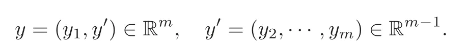
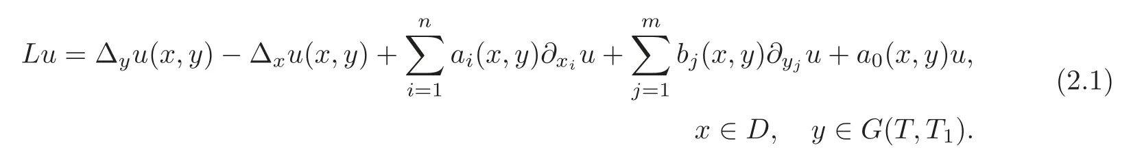
Letn,m∈N andx∈Rn,y∈Rm.We consider the ultrahyperbolic equation

in some bounded domain of(x,y)∈Rn×Rm.We set

and

Ifm=1,then(1.1)is a hyperbolic equation,wherey1is the time variable.Generally,it is considered that one time dimension is fundamentally important in describing many dynamic evolutions of physical quantities in the classical and quantum fields.Multiple times have been considered rarely,because it is widely believed to violate the causality and lead to the instability yielding that the phenomena under consideration are not deterministic in a usual physical sense.However,certain developments in the theoretical physics such as the string theory requireadditional dimensions for the time,and for related literature,we refer to Bars[4],Craig and Weinstein[11],Sparling[29],and Tegmark[31].In particular,the multiple dimensions are considered in the context of the twistor spaces(see[29]).
The quantum kinetic theory is one of the fields in which ultrahyperbolic type equations are arising.For example,let us consider the quantum kinetic equation:

in a domain{(x,p,t);x=whereu(x,p,t)is the quantum distribution function,his Planck’s constant,i is the imaginary unit, Φ(x,t)is the potential andf(x,p,t)is the function characterizing the sources.Applying the Fourier transform with respect topand the change of variables of the form

one can obtain the following ultrahyperbolic type equation:

wherew(ξ,η,t)=denote the Fourier transform ofuandfrespectively(see[2]).The ultrahyperbolic operator appears also as the stationary part of a generalized Schrdinger equation:

and for related nonlinear generalized Schrdinger equations,see[18–19,30].
The solutions of some direct problems to ultrahyperbolic equations were investigated by Kostomarov[24–25]in the case ofn=3,m=2 andn=3,m=3.As for the uniqueness and some mean value property of solutions to general ultrahyperbolic equations,see[10,12,14,27],but there are very few results on the existence of the solution.In[11],the unique existence of solutions was proved forwith suitably given initial data and also some non-uniqueness results were proved by some choice of hyperplanes,where the initial data are given.The proof in[11]assumed that all the coefficients in the ultrahyperbolic equation are constant in the whole domain because the key is the Fourier transform.There seems to be no result on the existence of the solution to a Cauchy problem of the ultrahyperbolic equation with non-analytic coefficients.In the case of analytic coefficients,by the Cauchy-Kovalevskaja theorem,we can establish the well-posedness of the initial value problem of determining the solutionuto(1.1)satisfyingwhereaandbare analytic.
In this article,we discuss inverse problems of determining a coefficient or a source term in an ultrahyperbolic equation.First we formulate an inverse source problem.
LetD⊂Rnbe a bounded domain with smooth boundary∂Dand let
We arbitrarily fix
Henceforth(·,·)means the scalar product in Rnand Rm.ForT,T1>0,we set

In particular,we write

Throughout this article,we identifyLetp(x,y′)be given,ν(x)=(ν1(x),···,νn(x))denote the unit outward normal vector to∂D,and∂νu=(∇xu,ν).Moreover,letT,T1>0 and Γ⊂∂Dbe given.We consider the following system:
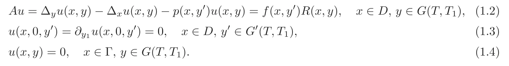
We consider an inverse problem of determiningf(x,y′)in(1.2)by extra data of the solution to(1.2)–(1.4).
Inverse Source ProblemLetp,Rbe given suitably.Then determinef(x,y′),x∈D,Here we do not assume the uniqueness ofu,but its existence.
Next we discuss an inverse problem of determining a coefficient by overdetermining lateral boundary data.More precisely,we consider
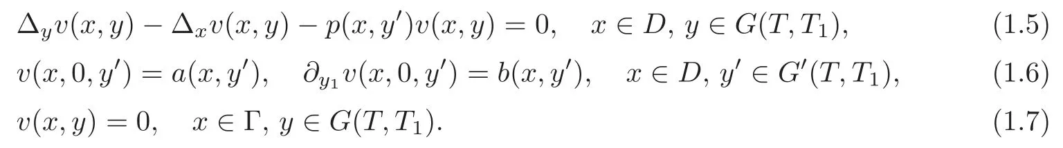
Letv=v(p)satisfy(1.5)–(1.7).We discuss the following problem.
Coefficient Inverse ProblemDetermine the coefficientin(1.5)by extra data
Our main purpose is to establish the uniqueness and the stability for these inverse problems,assuming the existence ofv(p)andv(q)within adequate classes.
The coefficient inverse problem is reduced to the inverse source problem as follows.Letv(p)andv(q)be two solutions of(1.5)–(1.7)with the coefficientspandqrespectively.Here we do not assume the uniqueness ofv(p)andv(q)but their existence.
The differenceu=v(p)−v(q)satisfies(1.2)–(1.4),whereandR=v(q)(x,y).Therefore the determination ofp,qis reduced to the inverse source problem.
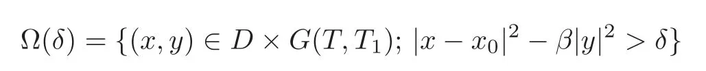
Thus we first discuss the inverse source problem for(1.2)–(1.4).For the statements of the main results,we introduce the following notations.Forδ>0,x0and 0<β<1,we define the domains by

We use the same notationsforG=if there is no fear of confusion.LetM>0 be arbitrarily fixed.
We are ready to state the following theorem.
Theorem 1.1We consider(1.2)–(1.3)in D×G.Let
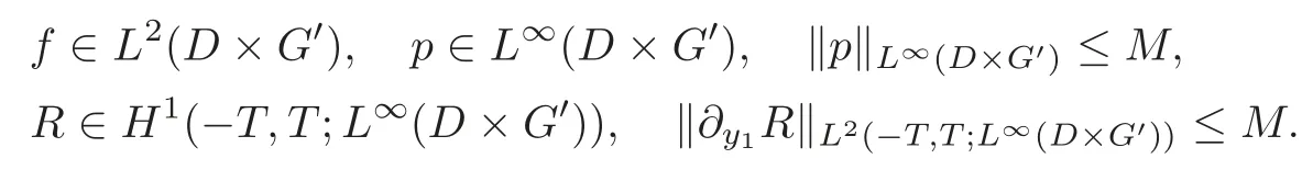
We further assume that

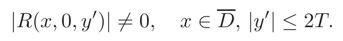
and that there exists a constant r0>0such that

Finally we assume

and thatΓ⊂∂D satisfies

Then for any δ1>δ,there exist constants C>0and θ∈(0,1),depending on M,r0such that

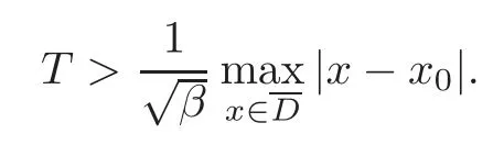
Theorem 1.1 gives a local estimate.More precisely,given Γ⊂∂DandT>0,we can find a subdomainwhere theL2-norm offis estimated.For example,we chooseδ>0 with> δand 0<t0<Tarbitrarily.We takeβsufficiently small such thatFor thisβ,we chooseT>0 sufficiently large such that(1.8)holds.Then Theorem 1.1 asserts

In fact,we chooseδ1>0 sufficiently close toδsuch thatSincefor|x−x0|<t0,we see thatTherefore(1.10)yields(1.11).
If we want to estimateffor largert0,thenβhas to be small and so we have to chooseT>0 very large,that is,we need to observe longer iny-direction as the right-hand side of(1.11)shows.In particular,for sufficiently largeδ1we haveand so the left-hand side of(1.11)estimatesfoverDprovided thatt0is small andT>0 is very large.The above observation means that if we want to estimatefin a larger subdomain ofD,then the sizeTof the “time” region has to be large.This fact corresponds to the finiteness of the propagation speed,which is a typical character for the case ofm=1.
In Theorem 1.1,it is not clear how largeTand Γ are necessary for identifyingfin a given subdomain orD×G′.Next we derive the estimation offin an arbitrarily given subdomain ofD×G′.For the statement,we recall

withT>0.Forwe set

We note that∂D+is a proper subset of∂Din general.
Theorem 1.2Let u satisfy(1.2)–(1.3)in D×G(T,2T)and u=0on∂D×G(T,2T)and

We further assume that β>0is sufficiently small and

and that

and
Then for any small>0,there exist constants C>0and θ∈(0,1)depending on,M,x0,such that

Next we show stability results for the coefficient inverse problem.We state two results which correspond to Theorems 1.1–1.2,respectively.
Theorem 1.3We consider(1.5)–(1.7).Let
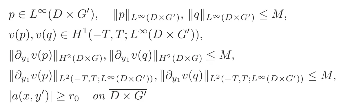
with some r0>0.We assume that0<β<1,(1.8)and(1.9)hold.Then for any δ1>δ,there exist constants C>0and θ ∈(0,1),depending on M,r0,such that

Theorem 1.4Let v(p),v(q)satisfy(1.5)–(1.6)with p,q respectively and v(p)=v(q)on∂D×G(T,2T).We assume
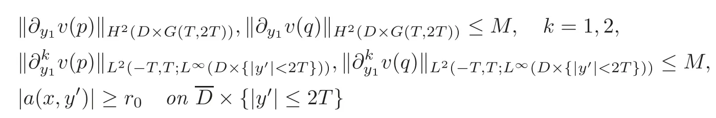
with some r0>0.We further assume
Then for any small>0,there exist constants C>0and θ∈(0,1)depending on,M,x0,such that

As is seen by the proof in Section 4,in Theorem 1.2,we can obtain the same stability in the case whereG(T,2T)is replaced by a smallerG:=if we can take also the norm of data on the other subboundary ofG:

whereνis the unit outward normal vector to∂GandA similar remark holds for Theorem 1.4.Moreover,if we have an a priori Lipschitz estimate for the direct problem for(1.2)–(1.3)withu=0 on(∂D×G)∪(D×then the same method as Imanuvilov and Yamamoto[16]can yield the Lipschitz stability,but we do not know such Lipschitz stability for the direct problem form≥2.In the case ofm=1,that is,the inverse hyperbolic problem,we can replace(1.15)by the Lipschitz stability(see[15–16])and we note that we need not fix>0.Moreover,for the uniqueness offinD×we need a boundary datum∂νuover∂D+×<2T},that is,we need a twice longery′-region for the observation than the domain iny′wherefis determined.
In Theorems 1.2 and 1.4,we can not take=0.However,since>0 is arbitrary,we can prove the uniqueness:For example,in Theorem 1.2,ifu(x,y)=0 forx∈ ∂D,|y1|<Tand<2Tand∂νu(x,y)=0 forx<2T,thenf(x,y′)=0 forx∈Dand
The proofs of the theorems are based on the method by Bukhgeim and Klibanov[9].In[9],the authors first applied a Carleman estimate which is anL2-estimate with large parameters,and then established the uniqueness in determining a spatially varying coefficient by overdetermining lateral boundary data.After[9],there have been many works relying on that method with modified arguments.We refer to Amirov[1–2],Amirov and Yamamoto[3],Baudouin and Puel[5],Bellassoued[6],Bellassoued and Yamamoto[7–8],Imanuvilov and Yamamoto[15–16],Isakov[17],Kha˘ıdarov[20],Klibanov[21–22],Klibanov and Timonov[23],and Yamamoto[32].Here we do not intend to give a complete list of the works and refer to the references therein.There are satisfactory amounts of works on classical equations in mathematical physics,but there are very few works for inverse problems of ultrahyperbolic equations.A key Carleman estimate was proved by Amirov[1–2]and Lavrent’ev,Romanov and Shishat·ski˘ı[26],where they applied the Carleman estimates to the unique continuation and proved stability.See also Romanov[28]for a Carleman estimate for an ultrahyperbolic equation in a Riemannian manifold and an application to some unique continuation problems.In Chapter 4 of Amirov[2],the uniqueness for an inverse source problem of a different type was proved by using the Carleman estimate.To the best knowledge of the authors,there are no results on the conditional stability like Theorems 1.1–1.4.
This paper is composed of four sections and one appendix.In Section 2,we present two Carleman estimates.Sections 3–4 are devoted to the proofs of Theorems 1.1–1.2 respectively.The proof of the key Carleman estimate is given in Appendix.
2 Key Carleman Estimate
In this section,we show two Carleman estimates for an ultrahyperbolic equation.The former Carleman estimate is used for the proof of Theorem 1.1 and the latter for the proof of Theorem 1.2.As for the general theory of Carleman estimates for functions with compact supports,we refer to,for example,Hrmander[13]and Isakov[17],but we here give a direct proof because we need a Carleman estimate for functions not having compact supports and the proof of that Carleman estimate does not follow directly from[13,17].Another direct proof of a Carleman estimate for an ultrahyperbolic equation is found in[2,26].
Here and henceforth let=D× ∂G(T,T1),and letand···dSybe the boundary integrals on Γxand Γy,respectively.
We recall that forwe set

whereγis a positive parameter.We consider the following equation:
Here we recall that
and

Letμ(x,y)be the outward unit normal vector to∂(D×G(T,T1))at(x,y)and letHenceforth we recall that∂D+⊂∂Dis defined by(1.13).
Theorem 2.1In(2.1),let us assume thatfor0≤i≤n and1≤j≤m.Moreover,let0<β <1be small and γ>0be sufficiently large,and let

with some δ0>0.Then there exist constants C>0and s0>0such that
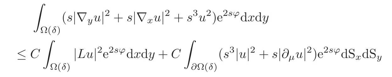
for all u∈H2(D×G(T,T1))and s≥s0.
Theorem 2.20≤i≤n,1≤j≤m and(2.2)hold for(x,y)∈D×G(T,T1).Then there exist constants C>0and s0>0such that

for all s≥s0and all u∈H2(D×G(T,T1))satisfying

Theorem 2.1 gives a Carleman estimate which holds only in a level set Ω(δ),while the Carleman estimate in Theorem 2.2 is global over the total domainG×(T,T1).The proofs of Theorems 2.1–2.2 rely on an idea similar to Bellassoued and Yamamoto[8]and the proof is obtained only by integration by parts and is lengthy,so we give the proof in Appendix.
3 Proof of Theorem 1.1
The proofs of Theorems 1.3–1.4 are reduced to the proofs of Theorems 1.1–1.2,respectively,which this follows from settingu=v(p)−v(q),f=p−qandR=v(q).Therefore it is sufficient to prove only Theorems 1.1–1.2.In this section,we will prove Theorem 1.1.
We set

First by(1.8),we see that

In fact,letx∈DandThen(1.8)yields

Therefore,0,that is,|y|<T.Thus(3.1)is verified.
Next,we characterize∂Ω(δ).We can easily have∂Ω(δ)

Then,similar to(3.1),we can prove that Γ2=Ø.In fact,(1.8)implies

which is impossible.
Moreover,noting thatwe see that

Hence

Now we apply the Carleman estimate in Theorem 2.1,but no data are given on

and so we need a cut-offfunction.
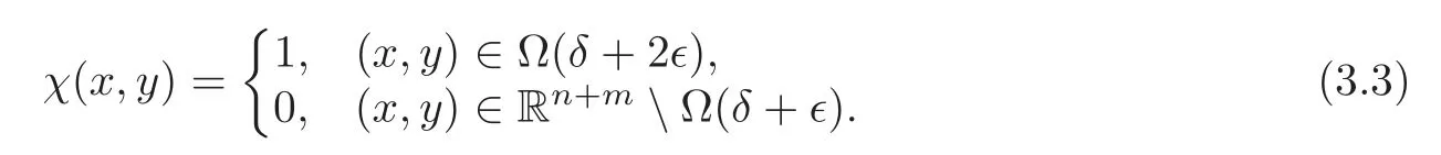
Henceforth,C>0 denotes a generic constant which is independent ofs.We define a cut-offfunctionsuch that 0≤χ(x,y)≤1 and
Settingz=for 1≤i≤n,we have
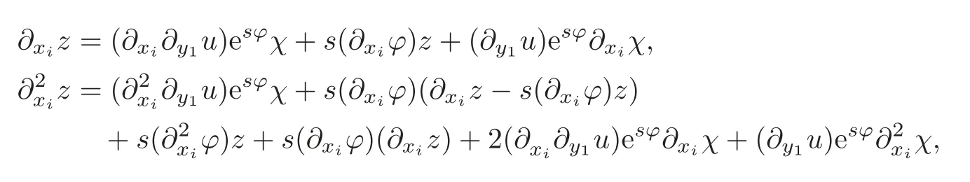
that is,

Similarly,

From(1.2),we obtain

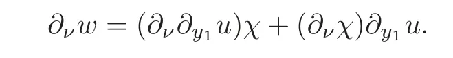
In particular,settingw=ands=0 in(3.4)we have

By(3.2)–(3.3),we see that

By(1.4)we have=0 andon Γ×G.Moreover,by 0<β<1 we note that

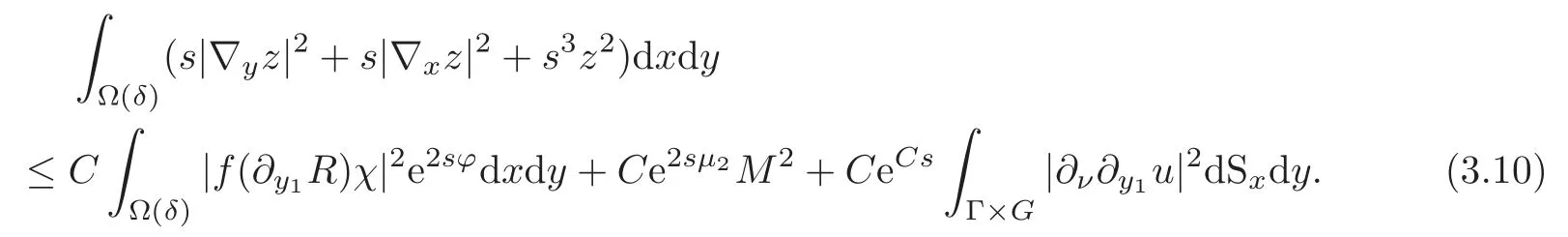
Thus the assumptions in Theorem 2.1 are satisfied in Ω(δ).We apply the Carleman estimate given by Theorem 2.1,and we obtain

Here we also used
Sincez=we have

and

We set

On the other hand,by(3.3),the supports of the functionsare the subsets ofso that

In terms of(3.7)–(3.9),we rewrite(3.6)as
We set
We multiply(3.4)byzand integrate it overto have

We denote the left-hand side of(3.11)by I1and the right-hand side by I2.By(3.2),we note that

Moreover,by(1.3)–(1.4)and(3.3),we have

and

Then,we have

Therefore,using the integration by parts,we obtain

Consequently,we have

Hereis the-component of the unit outward normal vectorνtoWe see that=0 on Γ×G.Moreover,=0 onTherefore,(3.12)yields

From(1.2),we have

Thus by(3.3)and the condition>0,we see that

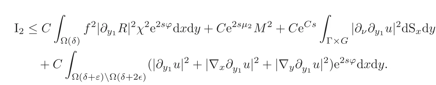
Next we estimate I2.Using the Cauchy-Schwarz inequality,we have

Therefore we absorb the terms includingdxdyintosdxdy,and we obtain

Now by noting that⊂Ω(δ),(3.3)and(3.10),we have
By(3.3)and the a priori boundedness onu,we have

and so

Now we will consider the first term on the right-hand side of(3.15).SinceandR(x,0,>0 onwe can define a function(−T,T)by
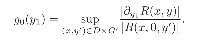
Then we can write

On the other hand,we have

In fact,let∈Ω(δ+2).Then

Hence(1.8)impliesand so

that is,|y1|<T.Since

we see that(x,0,+2).
Consequently we obtain

where

Moreover,(−T,T)and the Lebesgue theorem imply
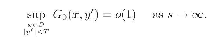
Henceforth,we set
Then(3.15)yields
From(3.14)and(3.16),we obtain

Finally

for all larges≥whereis some constant.Reducing the integral on the left-hand side to Ω′(δ+3),we have
that is,

for alls≥whereμ=−ReplacingCbywe see that(3.18)holds for alls≥0.First,letM≥d.Choosings≥0 such that
we obtain

Second,letM<d.Then settings=0 in(3.18),we have

Therefore

By the a priori boundedness≤Mand the trace theorem,we haved≤CMand so we can haveSince>0 is arbitrarily small,the proof of Theorem 1.1 is completed.
4 Proof of Theorem 1.2
The proof relies on Theorem 2.2 and is similar to that in[16].
Sinceuitself does not satisfy(2.3),we have to introduce a cut-offfunction.Moreover,we have to apply a Carleman estimate by shifting the domain along they′-direction.Thus we need to introduce several notations.We set

Bywe see thatr>0.We chooseρ>1 sufficiently large so that

By(4.1)and the assumption onT,we have

Furthermore,if necessary,we choose smallerβsuch that

We arbitrarily choose∈Rm−1satisfying
We set

and we recall
Moreover let

Then(4.2)yields

and

Therefore,for small>0 there existsδ>0 such that

ifT−2δ≤|y1|≤TorT−2δ≤≤Tand

In order to apply Theorem 2.2,we introduce a cut-offfunctionχ(y)and definesuch that 0≤χ0≤1 and
Setting=we see thatχ0≤χ≤1 and

By choosingδ>0 smaller if necessary,we assume
We set

Then

and
From(4.4),we note that

By(4.12)–(4.13),we can apply the Carleman estimate(see Theorem 2.2)tow1,w2:

Here and henceforth,C>0 denotes a generic constant which is independent ofs>0.From the assumption onR,we have

By(4.10),we see that|y1|≤T−2δorT−δ≤|y1|≤Timpliesχ=χ=0,and|y′−≤T−2δorT−δ≤|y′−≤Timpliesχ=χ=0 for 2≤k≤m.Therefore,if|y1|∈[0,T−2δ]∪[T− δ,T]and|y′−∈[0,T−2δ]∪[T−δ,T],then|∇yχ|=Δyχ=0.Hence

By(4.8),we haveψ(x,y)<−in the regions of the above integrals.Hence
Here and henceforth we set

Finally,we obtain

Here we used(4.14).
Consequently(4.15)yields

Next,sinceχ(−T,by(4.10),the Cauchy-Schwarz inequality yields

For the last inequality,we used(4.16)and

Hence

Applying(4.18),we have
Here we used≤1 andforx∈Dandy∈
On the other hand,substitutingy1=0 in(1.2)and applyingu(x,0,y′)=0 andR(x,0,y′)≠0forx∈and|y′|≤2T,we have

Noting by(4.4)that if<T,then|y′|<2T,we apply(4.20)in(4.19),so that

for all larges>0.Absorbing the first term on the right-hand side into the left-hand side by choosings>0 large,we obtain

for all larges>0.
Replacing the integration domain on the left-hand side byD×⊂D×and using(4.9)–(4.11),we see that=1 there and

for alls≥s0,wheres0is some constant.By the definition,we haveκ2>κ1and setκ=κ2−κ1>0.Then the last inequality implies
for alls≥s0.By the same argument as in the proof of Theorem 1.1 after(3.18),we can chooseθ∈(0,1)such that

for allsatisfying≤M,the trace theorem yieldsd≤CM,which impliesd≤Varyingand noting

we obtain

Thus the proof of Theorem 1.2 is completed.
5 Appendix
Thanks to the large parameters,it is sufficient to prove Theorems 2.1–2.2 in the case ofai=bj=0 in(2.1).Let us set

We prove only Theorem 2.2 and the proof of Theorem 2.1 is obtained by replacing the domainD×G(T,T1)by Ω(δ).Henceforth,we writeand useνto denote the unit outward normal vector to a hypersurface under consideration and we set∂νz=(∇xz,ν)or∂νz=(∇yz,ν).Moreover,we set

and

By(5.3),we calculate

where

The first term on the right-hand side of the Carleman estimate isand it suffices to make a lower estimation ofSince

we will estimateas follows.Using(5.5)–(5.6),we obtain
where
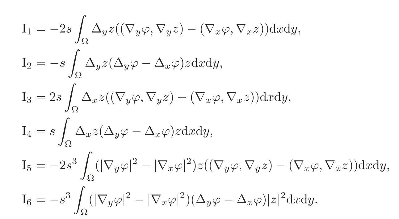
Now,we will estimate the terms Ik,1≤k≤6,using the integration by parts and the boundary condition ofz.Then we have


and

Therefore,we can rewrite

where

and

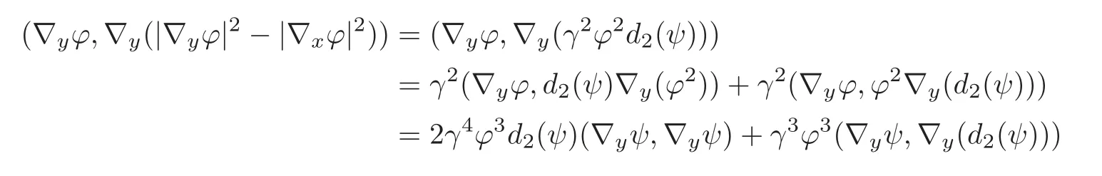
Next we calculate Jk,1≤k≤5 by substituting the concrete form ofϕ.Setting

we have

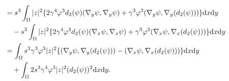
Therefore,we obtain

and

We can directly verify

In fact,


Consequently,we see that

Since
we have

We can directly verify
and

Therefore,we conclude that

Finally,we obtain the boundary term as follows:

Then from(5.7),we have

where


We haveϕ≥1 onand sok=1,2,3 onMoreover the second,third and fifth terms on the right-hand side of(5.9)are summed up into
Hence

By the assumption(2.2),we have

Therefore,we can write

In(5.10),the signs of the terms ofandare different.Thus we need to perform another estimation for
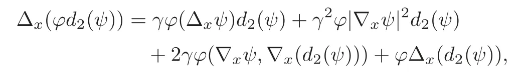
Multiplying the equationPz=byϕzand applying the integration by parts,we have

Now we estimate the terms Kj,1≤j≤5 as follows:

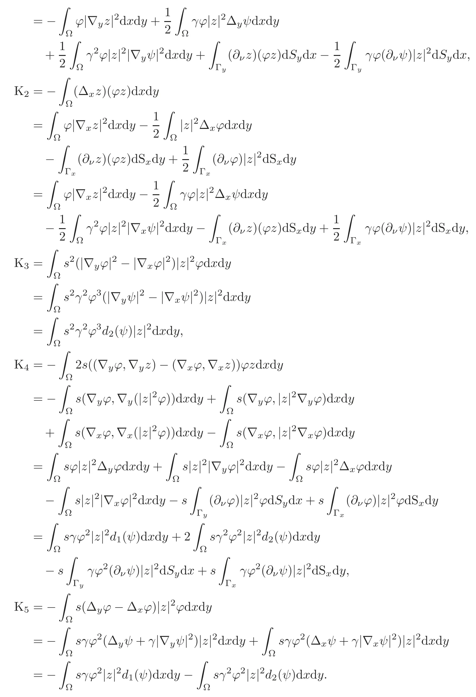
Therefore we see that


Here

becausez=0 onby(2.3).Now we calculate B0given by(5.8),while(2.3)implies∇yz=0 andon Γxand all the integrations on Γyvanish.Hence

So multiplying(5.11)by−sγ(4β+μ),where we chooseμ>0 later,we have
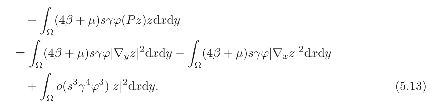
We add(5.10)and(5.13)to have

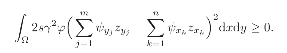
On the other hand,since
by the Cauchy-Schwarz inequality,we see

By 0<β<1,we can chooseμ>0 sufficiently small,so that

Absorbing the term ofwe complete the proof of Theorem 2.2.
AcknowledgmentThe authors thank the anonymous referees for valuable comments.
[1]Amirov,A.K.,Doctoral Dissertation in Mathematics and Physics,Sobolev Institute of Mathematics,Novosibirsk,1988.
[2]Amirov,A.K.,Integral Geometry and Inverse Problems for Kinetic Equations,VSP,Utrecht,2001.
[3]Amirov,A.K.and Yamamoto,M.,A timelike Cauchy problem and an inverse problem for general hyperbolic equations,Appl.Math.Lett.,21,2008,885–891.
[4]Bars,I.,Survey of two-time physics,Class.Quantum Grav.,18,2001,3113–3130.
[5]Baudouin,L.and Puel,J.-P.,Uniqueness and stability in an inverse problem for the Schrdinger equation,Inverse Problems,18,2002,1537–1554.
[6]Bellassoued,M.,Uniqueness and stability in determining the speed of propagation of second-order hyperbolic equation with variable coefficients,Applicable Analysis,83,2004,983–1014.
[7]Bellassoued,M.and Yamamoto,M.,Logarithmic stability in determination of a coefficient in an acoustic equation by arbitrary boundary observation,J.Math.Pures Appl.,85,2006,193–224.
[8]Bellassoued,M.and Yamamoto,M.,Carleman estimate with second large parameter for second order hyperbolic operators in a Riemannian manifold and applications in thermoelasticity cases,Applicable Analysis,91,2012,35–67.
[9]Bukhgeim,A.L.and Klibanov,M.V.,Global uniqueness of a class of multidimensional inverse problems,Soviet Math.Dokl.,24,1981,244–247.
[10]Burskii,V.P.and Kirichenko,E.V.,Unique solvability of the Dirichlet problem for an ultrahyperbolic equation in a ball,Differential Equations,44,2008,486–498.
[11]Craig,W.and Weinstein,S.,On determinism and well-posedness in multiple time dimensions,Proc.Royal Society A,465,2009,3023–3046.
[12]Diaz,J.B.and Young,E.C.,Uniqueness of solutions of certain boundary value problems for ultrahyperbolic equations,Proc.Amer.Math.Soc.,29,1971,569–574.
[13]Hrmander,L.,Linear Partial Differential Operators,Springer-Verlag,Berlin,1963.
[14]Hrmander,L.,Asgeirsson’s mean value theorem and related identities,J.Funct.Anal.,184,2001,377–401.
[15]Imanuvilov,O.Y.and Yamamoto,M.,Lipschitz stability in inverse parabolic problems by the Carleman estimate,Inverse Problems,14,1998,1229–1249.
[16]Imanuvilov,O.Y.and Yamamoto,M.,Global Lipschitz stability in an inverse hyperbolic problem by interior observations,Inverse Problems,17,2001,717–728.
[17]Isakov,V.,Inverse Problems for Partial Differential Equations,Springer-Verlag,Berlin,2006.
[18]Kenig,C.E.,Ponce,G.,Rolvung,C.and Vega,L.,Variable coefficient Schrdinger flows for ultrahyperbolic operators,Advances in Mathematics,196,2005,373–486.
[19]Kenig,C.E.,Ponce,G.and Vega,L.,Smoothing effects and local existence theory for the generalized nonlinear Schrdinger equations,Inven.Math.,134,1998,489–545.
[20]Khaıdarov,A.,On stability estimates in multidimensional inverse problems for differential equation,Soviet Math.Dokl.,38,1989,614–617.
[21]Klibanov,M.V.,Inverse problems in the “ large” and Carleman bounds,Differential Equations,20,1984,755–760.
[22]Klibanov,M.V.,Inverse problems and Carleman estimates,Inverse Problems,8,1992,575–596.
[23]Klibanov,M.V.and Timonov,A.,Carleman Estimates for Coefficient Inverse Problems and Numerical Applications,VSP,Utrecht,2004.
[24]Kostomarov,D.P.,A Cauchy problem for an ultrahyperbolic equation,Differential Equations,38,2002,1155–1161.
[25]Kostomarov,D.P.,Problems for an ultrahyperbolic equation in the half-space with the boundedness condition for the solution,Differential Equations,42,2006,261–268.
[26]Lavrent’ev,M.M.,Romanov,V.G.and Shishat·skiı,S.P.,Ill-posed Problems of Mathematical Physics and Analysis,American Math.Soc.,Providence,RI,1986.
[27]Owens,O.G.,Uniqueness of solutions of ultrahyperbolic partial differential equations,Amer.J.Math.,69,1947,184–188.
[28]Romanov,V.G.,Estimate for the solution to the Cauchy problem for an ultrahyperbolic inequality,Doklady Math.,74,2006,751–754.
[29]Sparling,G.A.J.,Germ of a synthesis:space-time is spinorial,extra dimensions are time-like,Proc.Royal Soc.A,463,2007,1665–1679.
[30]Sulem,C.and Sulem,P.-L.,The Nonlinear Schrdinger Equation,Spriner-Verlag,Berlin,1999.
[31]Tegmark,M.,On the dimensionality of space-time,Class.Quant.Grav.,14,1997,L69–L75.
[32]Yamamoto,M.,Carleman estimates for parabolic equations and applications,Inverse Problems,25,2009,123013,75 pages.
 Chinese Annals of Mathematics,Series B2014年4期
- Chinese Annals of Mathematics,Series B的其它文章
- Poles of L-Functions on Quaternion Groups
- The∂-Stabilization of a Heegaard Splitting with Distance at Least 6 is Unstabilized∗
- Monomial Base for Little q-Schur Algebra uk(2,r)at Even Roots of Unity
- Delay-Dependent Exponential Stability for Nonlinear Reaction-Diffusion Uncertain Cohen-Grossberg Neural Networks with Partially Known Transition Rates via Hardy-Poincar´e Inequality∗
- Betti Numbers of Locally Standard 2-Torus Manifolds∗
- Random Sampling Scattered Data with Multivariate Bernstein Polynomials∗