Delay-Dependent Exponential Stability for Nonlinear Reaction-Diffusion Uncertain Cohen-Grossberg Neural Networks with Partially Known Transition Rates via Hardy-Poincar´e Inequality∗

Ruofeng RAO

1 Introduction

It is well-known that Cohen-Grossberg in[1]proposed originally the CGNNs.Since then the CGNNs have founded its extensive applications in pattern recognition,image and signal processing,quadratic optimization,and aritifical intelligence(see[2–11]).However,these successful applications are greatly dependent on the stability of the neural networks,which is also a crucial feature in the design of the neural networks.In practice,both time delays and impulse are always inevitable,and cause probably some undesirable dynamic network behaviors such as oscillation and instability.Therefore,the stability analysis for delayed impulsive CGNNs has become a topic of great theoretic and practical importance in recent years(see[2–3,5–6]).Recently,the CGNNs with Markovian jumping parameters have been extensively studied,for the systems with Markovian jumping parameters are useful in modeling abrupt phenomena,suchas random failures,operating in different points of a nonlinear plant,and changing in the interconnections of subsystems(see[5–8]).Noise disturbance is unavoidable in real nervous systems,which is a major source of instability and poor performances in neural networks.A neural network can be stabilized or destabilized by certain stochastic inputs.The synaptic transmission in real neural networks can be viewed as a noisy process introduced by random fluctuations from the release of neurotransmitters and other probabilistic causes(see[12]).Hence,noise disturbance should be also taken into consideration in discussing the stability of neural networks(see[13–17]).On the other hand,diffusion phenomena can not be unavoidable in real world.Usually diffusion phenomena is simulated by linear Laplace diffusion for simplicity in many previous literatures(see[2,18–20]).However,diffusion behavior is so complicated that the nonlinear reaction-diffusion models were considered in several papers(see[3,21–24]).Even the nonlinearp-Laplace diffusion(p＞1)was considered in simulating some diffusion behaviors(see[3,6,10]).Particularly,ifp=2,thep-Laplace diffusion was just the conventional linear Laplace diffusion in many previous papers(see[2,18–20]).In addition,neural networks may encounter various other factors and problems in the factual operations.In fact,there exist also parameter errors unavoidable in factual systems owing to aging of electronic component,external disturbance and parameter perturbations.It is equally important to ensure that system is stable with respect to these uncertainties(see[25–26]).Naturally,aging of electronic component,external disturbance and parameter perturbations always result in a side-effect of partially unknown Markovian transition rates.Some of recent literatures investigated the stability of neural networks with partially unknown Markovian transition rates(see[27–28]).As far as we know,stochastic stability for the delayed impulsive Markovian jumping Laplace diffusion CGNN with uncertain parameters has rarely been considered.Besides,the stochastic exponential stability always remains the key factor of concern owing to its importance in designing a neural network,and such a situation motivates our present study.Motivated by the above-mentioned literature,particularly by[2,29–30],we shall investigate the stochastic global exponential stability criteria for the above-mentioned CGNN via the LMIs approach.

The rest of this paper is organized as follows.In Section 2,new CGNN models are formulated,and some preliminaries are given.In Section 3,new LMI-based stochastic global exponential stability criterion are presented for the CGNNs.And in Section 4,three numerical examples are provided to show the higher feasibility and less conservatism of the new criterion compared with those of[2–3,29–30].Finally,some conclusions are presented in Section 5.

2 Model Description and Preliminaries

In 2011,Zhang,Wu and Li in[2]considered the following Cohen-Grossberg neural networks under Dirichlet boundary condition:

whereu=u(t,x)=(u1(t,x),u2(t,x),···,un(t,x))T,=,···,=···,

Generally,there exist the following assumptions for the system(2.1)(see[2]):

(H1)u(t,x))is a bounded,positive and continuous diagonal matrix,i.e.,there exist two positive definite diagonal matricessuch that 0＜A≤

(H2)(u(t,x))=,···,such that there exists a positive definite matrix=diag(satisfying

(H3)There exist diagonal matrices

such that

and

In this paper,we always assume≡0 for some rational reason(see Remark 2.3),and consider to replace(H3)with the following more flexible condition:

(H3*)There exist constant diagonal matrices

with

such that

According to[2,Definition 2.1],a constant vectoru∗∈Rnis said to be an equilibrium point of system(2.1)if

Letv=u−u∗,then the system(2.1)with~h≡0 can be transformed into

wherev=v(t,x)=···,u∗=A(v(t,x))=(v(t,x)+u∗)=(u(t,x)),

and

Then,according to[2,Definition 2.1],v≡0 is an equilibrium point of system(2.4).Hence,below we only need consider the stability of the null solution of Cohen-Grossberg neural networks.Naturally we propose the following hypotheses on the system(2.4)withh≡0,which are perhaps derived by the assumptions(H1)–(H2)and(H3*).

(A1)A(v(t,x))is a bounded,positive and continuous diagonal matrix,i.e.,there exist two positive diagonal matricesandsuch that 0＜≤A(v(t,x))≤

(A2)B(v(t,x))=,···,,such that there exists a positive definite matrixB=diag(B1,B2,···,Bn)T∈Rnsatisfying

(A3)There exist constant diagonal matrices

withj=1,2,···,n,such that

Remark 2.1In many previous literatures,e.g.[2],authors always assume

which may be correspond to(H3).However,in(A3)may not be positive constants,and hence the functionsf,gare more generic.

Remark 2.2It is obvious from(2.5)thatB(0)=0=f(0)=g(0),and thenB(0)−Cf(0)−Dg(0)=0.

Very recently,Wang,Rao and Zhong[3]studied stochastic CGNN with nonlinearp-Laplace diffusion(p＞1)under Neumann boundary condition:

Since stochastic noise disturbance and parameter errors are unavoidable in the practical neural networks,it is necessary to consider the stability of the null solution of the following Markovian jumping CGNN:

The initial conditions and the boundary conditions are given by

and

respectively,wherep＞1 is a given scalar,and Ω∈Rmis a bounded domain with a smooth boundary∂Ω of classC2by Ω,v(t,x)=···,∈Rn,wherevi(t,x)is the state variable of theith neuron at timetand in space variablex.MatrixD(t,x,v)=satisfies(t,x,v)≥d＞0 for allj,k,(t,x,v),where the smooth functionsare diffusion operators.Similarly as that of[3],we denoteAnd D(t,x,v)◦ ∇pv=denotes the Hadamard product of matrixD(t,x,v)and∇pv.For matrix Y=(Y1,···,Yn)TwithYi=(i=1,2,···,n),we denote∇·Y=(∇·Y1,∇·Y2,···,∇·Yn)T,where∇·Particularly,∇pv=∇vifp=2.

Denotew(t)=,···,,where(t)is scalar standard Brownian motion defined on a complete probability space(Ω∗,F,P)with a natural filtrationNoise perturbationsσ:R+×Rn×Rn×S→is a Borel measurable function.{r(t),t≥0}is a right-continuous Markov process on the probability space which takes values in the finite spaceS={1,2,···,s}with the generator Π =given by

where≥0 is transition probability rate fromitoj(j/i)and＞0 and=0.In addition,the transition rates of the Markovian chain are considered to be partially available,namely,some elements in transition rates matrix Π are time-invariant but unknown.For instance,a system with three operation modes may have the transition rate matrix Π as follows:

where “”represents the inaccessible element.For natation clarity,we denoteS=withis known}andis unknown,andji}for a giveni∈S.DenoteThe time-varying delayτ(t)satisfies 0≤ τ(t)≤ τwitht)≤ κ ＜1.

whereaj(vj(t,x))represents an amplification function,andis an appropriately behavior function.C(r(t),t),D(r(t),t)are denoted byCi(t),Di(t)withCi(t)==respectively,anddenote the connection strengths of thekth neuron on thelth neuron at timetin the moder(t)=i,respectively.Denote vector functionsf(v(t,x))=···,g(v(t,x))=···,whereare neuron activation functions of thejth unit at timetand in space variablex.

For any moder(t)=i∈S,we assume thatCi,Diare real constant matrices of appropriate dimensions,andare real-valued matrix functions which represent time-varying parameter uncertainties,satisfying

In addition,we always assume thatt0=0,and=v(,x)for allk=1,2,···,wherev(,x)andv(,x)represent the left-hand and right-hand limits ofv(t,x)at,respectively.And each(k=1,2,···)is an impulsive moment,satisfying 0＜t1＜t2＜···＜tk＜···and limtk=+∞.The boundary condition(2.7c)is called Dirichlet boundary condition if and Neumann boundary condition if B[(t,x)]=denotes the outward normal derivative on∂Ω.It is well-known that the stability of neural networks with Neumann boundary condition has been widely studied.The Dirichlet boundary conditions describe the situation,where the space is totally surrounded by a region in which the states of the neuron equal zero on the boundary.And the stability analysis of delayed reaction-diffusion neural networks with the Dirichlet boundary conditions is very important in theories and applications,and also has attracted much attention(see[2,31–34]).So in this paper,we consider the CGNN under Neumann boundary condition and Dirichlet boundary condition,respectively.

Remark 2.3If all stochastic factors and uncertain factors are ignored,the system(2.7)withp=2 was studied by[2]though there is a little difference between Dirichlet boundary condition and Neumann boundary condition.However,our impulsive assumptionis more natural than that of[2],which will result in some difference in methods(see,e.g.[3]).

Particularly,ifp=2,the system(2.7)is reduced to the following CGNN:

For convenience’s sake,we need introduce some standard notations.

(1)L2(R×Ω):The space of real Lebesgue measurable functions of R×Ω,it is a Banach space for the 2-norm‖v(t)‖2=where|·|is the Euclid norm.

(2)The family of allF0-measurableC([−τ,0]×Ω;Rn)-value random variableξ={ξ(θ,x):−τ≤θ≤0,x∈Ω}such that＜∞,where E{·}stands for the mathematical expectation operator with respect to the given probability measureP.

(3)Q=＞0(＜0):A positive(negative)definite matrix,i.e.,yTQy＞0(＜0)for any 0/y∈Rn.

(4)Q=≥0(≤0):A semi-positive(semi-negative)definite matrix,i.e.,yTQy≥0(≤0)for anyy∈Rn.

盖尔达耶属于炎热的沙漠气候，夏天极热，冬天温和，昼夜温差很大，夏季和冬季为5～46℃不等。夏天的风干燥、炎热而强烈，冬天的风温暖而干燥。全年降雨量极少，总量仅为75mm，夏季炎热季节降雨量最少，全年有降雨的天数不足24d，导致7月份的相对湿度仅为22.3%，1月份达到54.7%，全年大部分时间干燥炎热。此外，每年3～5月是沙尘暴肆掠的季节。

(5)This meansis a semi-positive(semi-negative)definite matrix.

(6)This meansis a positive(negative)definite matrix.

(7)denote the largest and the smallest eigenvalues of matrix Φ,respectively.

(8)Denote|C|=for any matrixC=

for anyu(t,x)=(u1(t,x),u2(t,x),···,un(t,x))T.

(9)I:Identity matrix with compatible dimension.

(10)The symmetric terms in a symmetric matrix are denoted by∗.

Throughout this paper,we assume(A1)–(A3)and the following conditions hold:

(A4)For any modei∈S,the parameter uncertainties considered here are norm-bounded and of the following forms:

whereK(t)is an unknown matrix function satisfyingare known real constant matrices.

(A5)There exist symmetrical matricesRj≥0 withj=1,2,such that for any modei∈S,

(A6)σ(t,0,0,i)=0 for alli∈S.

Remark 2.4The condition|H|=His not too stringent for a semi-positive definite matrixH=0.Indeed,allhij≥0 imply|H|=H.

Similarly as that of[2,Definition 2.1],we can see from(A6)that the system(2.7)has the null solution as its equilibrium point.Letv(t,x;φ,i0)be the state trajectory from the initial conditionr(0)=on−τ≤θ≤0 inBelow,we always assume thatv(t,x;φ,i0)is a solution of system(2.7).

Definition 2.1For any given scalar p＞1,the null solution of system(2.7)is said to be stochastically globally exponentially stable in the mean square if for every initial condition φ∈r(0)=i0,there exist scalars β＞0and γ＞0such that for any solution v(t,x;φ,i0),

Notice that ifp=2,the system(2.7)is just the system(2.9).And the following Poincar´e inequality lemma and Hardy-Poincar´e inequality lemma may play role in judging the stability of system(2.9).

Lemma 2.1(see[35])(PoincarInequality)LetΩbe a bounded domain ofRmwith a smooth boundary∂Ωof class C2byΩ.ψ(x)is a real-valued function belonging to(Ω)and satisfiesB[ψ(x)]|∂Ω=0.Then

where λ1is the lowest positive eigenvalue of the boundary value problem

Notice that(Ω)is the Sobolev spacewithp=2,andis the completion of(Ω)with respect to the normThereby,the norm ofNote that we always denote theL2(Ω)-norm by‖ψ‖=

Lemma 2.2(see[36])(Hardy-PoincarInequality)For any bounded domainΩinRm,any dimension m≥2and for every ψ(x)∈(Ω),we have

where the constantΛ2is the first eigenvalue of the Laplacian in the unit ball in m=2,and ωm denotes the measure of the unit ball inRm.

Lemma 2.3be a positive definite matrix for a given i,and v be a solution of system(2.7).Then we have

ProofSincevis a solution of system(2.7),we can see it by Gauss formula and Dirichlet or Neumann boundary condition that

Similarly,we can prove

Lemma 2.4(see[37])Let ε＞0be any given scalar,and M,Eand K be matrices with appropriate dimensions.If KTK≤I,then we have

3 Main Results

In order to compare with the main results of[2],we may give a prior consideration on the conventional linear Laplace diffusion system(2.9).

Theorem 3.1The null solution of system(2.9)is stochastically globally exponential stable in the mean square if there exist positive scalars λ≤λ1,β＞0,a sequence of positive scalarsand positive definite diagonal matricesand Q such that the following LMI conditions hold:

where

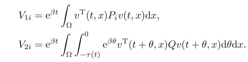
ProofConsider the Lyapunov-Krasovskii functional

where

Then by Itformula,we get the following stochastic differential:

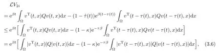
Lis the weak infinitesimal operator such thatLV(t,v(t,x),i)=for any giveni∈S.Next,it follows by Lemma 2.3(p=2)and(2.9)that forttk,

Here,v=v(t,x)is a solution of system(2.9).And fort/tk,

Moreover,we can get by Poincarinequality and 0＜λλ1,

It follows by(A1)–(A2)that

In addition,we have

Similarly,

From(A3),we have

Fromπii＜0 and the definition ofit is clear that

(A5)derives

Combining(3.5)–(3.14)results in

where

andζ(t,x)=(|vT(t,x)|,|vT(t−τ(t),x)|,|fT(v(t,x))|,|gT(v(t−τ(t),x))|)T.

Next we claim that Ai＜0.

For convenience,we denote

By applying Schur complement to(3.1),we can get from Lemma 2.4,

which proves our claim.And thenLV(t,v(t,x),i)≤0.Define

Then we haveV(t,v(t,x),i)=eβtV(t,v(t,x),i),satisfying

Now,by applying the Dynkin formula,we can derive that for anyi∈S,

In fact,due tov(,x)=v(tk,x),we might as well assume≤t＜tkfor any givenk∈{1,2,···}.And then we have

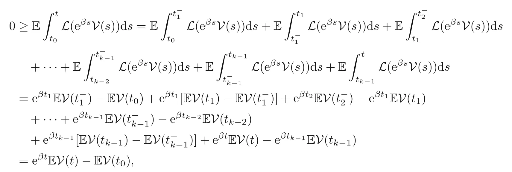
which proves(3.16).On the other hand,we claim

Indeed,we can get by the assumptions onMjk:

Thus,we prove the claim(3.17).Owing to(3.16)–(3.17),we get

Hence,combining(3.16)and(3.18)implies

Now,for anyφ(θ,x)([−τ,0]×Ω;Rn)and any system modei∈S,the solutionv(t,x,φ,i0)of system(2.9)with the initial valueφsatisfies

or

where scalarsγ=＞0,β＞0.Therefore,we can see it by(3.21)and Definition 2.1 that the null solution of system(2.9)is globally stochastically exponentially stable in the mean square.

Remark 3.1In Theorem 3.1,the magnitude ofλ1is determined by the bounded domain Ω∈Rm.However,ifm≥3,the exact computation ofλ1is usually not possible.Nevertheless,we can estimate the value ofλ1.For instance,under the Dirichlet boundary assumption,we may fixλ=in Theorem 3.1 due to Hardy-Poincar´e inequality.In fact,fromλ1=we know that 0＜λ≤λ1,satisfyingfor allψ∈(Ω).In many recent literatures(see[2,31–34]),Ω∈Rmis restricted to be a cube.Moreover,in their numerical examples,the dimensionmis restricted to be 1 or 2.Now,in this paper,we abolish these limitations thanks to the synthetic application of Poincarinequality and Hardy-Poincarinequality.Below,Example 4.3 will show the effectiveness of Theorem 3.1,where Ω is assumed to be a spheroid and not a sphere.Notice that if Ω is a ball,the constants of Hardy-Poincar´e inequality are optimal(see[36,Theorem 4.1]).But Theorem 3.1 admits actuallyλ＜λ1,and then we may fixλ=So we need not assume in numerical examples that Ω is the similar ball as that of[29–30].To the best of our knowledge,it is the first time to apply both Poincarinequality and Hardy-Poincar´e inequality to stability analysis of the reaction-diffusion neural networks.

Remark 3.2Below,Example 4.3 is given to show that Theorem 3.1 is more effective and less conservative than some existing results due to significant improvement in the allowable upper bounds of delays.

IfD(t,x,v)≡Dis a diagonal constant matrix,the system(2.9)is perhaps reduced to the following system:

where Δv(t,x)=(Δv1(t,x),Δv2(t,x),···,Δvn(t,x))T,and Δvj(t,x)

Similarly to(3.7),we have

where both constant matricesD=diag(D11,D22,···,Dnn)andP=diag(p11,p22,···,pnn)are positive definite.

Hence,similarly to the proof of Theorem 3.1,we can prove the following similar result.

Theorem 3.2The null solution of system(3.22)is stochastically globally exponential stable in the mean square if there exist positive scalars λ≤λ1,β＞0,a sequence of positive scalars(i∈S)and positive definite diagonal matrices Pi=diag(pi1,pi2,···,pin)(i∈S),L1,L2and Q such that the following LMI conditions hold:

where

Consider the deterministic system(2.4)withh≡0,

Then,from Theorem 3.2,we can deduce the following corollary.

Corollary 3.3The null solution of system(3.23)is stochastically globally exponential stable in the mean square if there exist positive scalars λ≤λ1,β＞0,and positive definite diagonal matrices P,L1,L2and Q such that the following LMI conditions hold:

where

Remark 3.3In[2,Theorem 3.1], Ω is restricted to be a cube Ω ={(x1,x2,···,xm)T∈Rm:|xj|＜lj,j=1,2,···,m},andF1=G1are assumed to be 0.Under the Dirichlet boundary condition,the null solution of system(3.23)is exponentially stable if all(C1)–(C3)(see[2,Theorem 3.1])are satisfied,where

andlHere,we point out that in comparison with Corollary 3.3,conditions(C1)–(C3)(see[2,Theorem 3.1])are too complicated to be satisfied.LMI condition(3.24)is more feasible than(C1)of[2,Theorem 2.1].Below we shall give a numerical example for it(see Example 4.1).

Finally,we consider the LMI criterion for the system(2.7)withp-Laplace diffusion(p＞1).

Theorem 3.4The null solution of system(2.7)is stochastically globally exponential stable in the mean square if there exists a positive scalar β＞0,a sequence of positive scalarsS)and positive definite diagonal matrices Pi=(i∈S),L1,L2and Q such that the following LMI conditions hold:

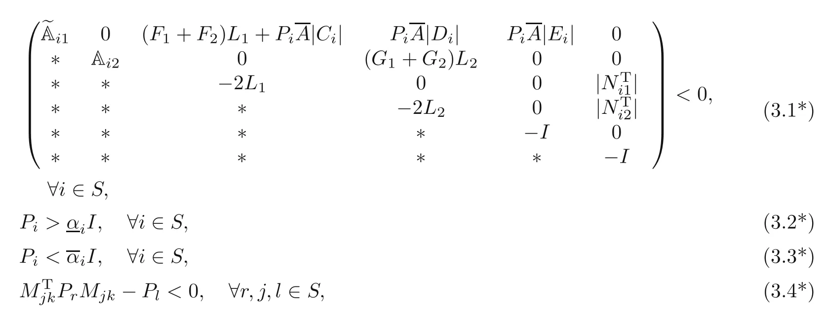
where

ProofFirst,we may construct the same Lyapunov-Krasovskii functional as that of the proof for Theorem 3.1.Second,we can get by Lemma 2.3:

And then we have the similar inequality as(3.5):

The rest of the proof is completely similar as that of Theorem 3.1.We can derive those similar inequalities as(3.6)–(3.21).And then,based on Definition 2.1,the null solution of system(2.7)is globally stochastically exponentially stable in the mean square.

If Markovian jumping phenomena and parametric uncertainties are ignored,the system(2.7)is reduced to the following system:

Then we get the following lemma from Theorem 3.4.

Corollary 3.5The null solution of system(3.26)is stochastically globally exponential stable in the mean square if there exist positive scalars β＞0,and positive definite diagonal matrices P,L1,L2and Q such that the following LMI conditions hold:

where

Remark 3.4In[3,Theorem 2.1],R2in(2.10)is assumed to be 0.In addition,F1=G1is also assumed to be 0.If there exist positive definite diagonal matricesP1,P2such that the following LMI holds:

and other two complicated conditions similar to(C2)and(C3)in[2,Theorem 3.1].Below,Example 4.2 shows that Corollary 3.5 is better than[3,Theorem 2.1]due to less conservativeness and more feasibility.

Remark 3.5The nonlinearp-Laplace diffusions in Theorem 3.4 bring a great difficulty establishing LMI conditions for the stability criterion.However,it is the first attempt to present the LMI-based criterion for the uncertain CGNNs with nonlinearp-Laplace diffusion.Below,Example 4.3 is given to show that Theorem 3.4 possesses less conservatism due to significant improvement in the allowable upper bounds of delays.

4 Numerical Examples and Comparisons

In this section,we shall give three numerical examples(Examples 4.1–4.3)for Corollaries 3.3 and 3.5 in comparison with[2,Theorem 3.1]and[3,Theorem 2.1].Finally,Example 4.3 is presented to illustrate that Theorems 3.1 and 3.4 possess more effectiveness and less conservatism due to significant improvement in the allowable upper bounds of delays.

Example 4.1Comparing Corollary 3.3 with the main result of[2].

Under the Dirichlet boundary condition,we consider the following system:

wherev=∈R2,Ω=:|xj|＜j=1,2},and thenl=1,λ1=π2=9.8696(see[35]).In addition,a1(v1)=0.13+0.07a2(v2)=0.14+0.06cos2(tx2),b1(v1)=0.02v1+2v1b2(v2)=0.016v2+12v2sin2(t2+x2),f(v)=g(v)=(0.1v1,0.1v2+0.1v2sin2(tx2))T,and

and hence

We might as well assume thatλ=9.8＜λ1,β=0.01,=0.525,τ(t)≡0.65=τand thenκ=0 for allt≥t0.We may takeλ=9.8.Now,by using Matlab LMI toolbox to solve the LMI(C1),we gettmin=0.0144＞0,which implies the LMI(C1)is found infeasible.But by using Matlab LMI toolbox to solve the LMIs(3.24)and(3.25),the result istmin=−0.1182＜0,and

Hence,Corollary 3.3 derives that the null solution of system(4.1)is stochastically globally exponential stable in the mean square(see Figures 1–3).

Figure 1 Computer simulations of the states v1(t,x)and v2(t,x)

Remark 4.1The stability of the null solution of system(4.1)can not be judged by[2,Theorem 3.1],for the first LMI(C1)of three conditions(C1)–(C3)is found infeasible.But all LMI conditions are only sufficient ones,not necessary for the stability.Corollary 3.3 shows that the null solution of system(4.1)is stochastically globally exponential stable in the mean square.Hence,Corollary 3.3 is really effective and less conservative than[2,Theorem 3.1].

Example 4.2Comparing Corollary 3.5 with the main result of[3].

Under the Neumann boundary condition and the initial condition(4.2),we consider the system(3.26)with the following parameters:

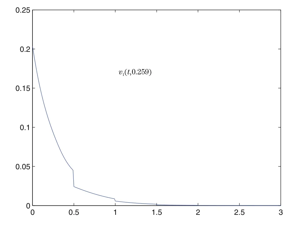
Figure 2 Sectional curve of the state variable v1(t,x)

Figure 3 Sectional curve of the state variable v2(t,x)

Assume,in addition,β=0.01,τ=0.65,k=0.

By using Matlab LMI toolbox to solve the LMI(C1*),the result istmin=0.0050＞0,which implies the LMI(C1*)is found infeasible.But by solving LMIs(3.1**)–(3.4**),one can obtaintmin=−0.0037＜0,and=2.1189,=7.6303,

Hence,Corollary 3.5 derives that the null solution of system(3.26)is stochastically globally exponential stable in the mean square.

Remark 4.2The stability of the null solution of system(3.26)with the above mentioned data can not be judged by[3,Theorem 2.1],for the first LMI(C1)of three conditions(C1)–(C3)is found infeasible.But all LMI conditions are only sufficient ones,not necessary for the stability.Hence,Corollary 3.5 is really more effective and less conservative than[3,Theorem 2.1]for the same reason as that of Remark 4.1.

Example 4.3Comparing the allowable upper bound of Theorem 3.1(p＞1)with that of Theorem 3.4(p=2).

Under the Dirichlet boundary condition,we consider the system(2.7)with the following parameters:

The transition matrix is considered as

Then we haved=0.003,0.7.Assume,in addition,β=0.01.Denotev=v(t,x)=(v1(t,x),v2(t,x))T,andx=∈Ω=A direct computation yields Λ2=5.7832,meas(Ω)=4.8842,and thenλ==5.2203.

Letτ(t)≡100.29,and thenκ=0.Now we use the Matlab LMI toolbox to solve the LMIs(3.1∗)–(3.4∗).The results showtmin=−0.0418＜0,and=1.8714,=0.7246,=1.9114,=0.7669,=1.8892,=0.7450,

Then we can conclude from Theorem 3.4 that the null solution of system(2.7)is stochastically globally exponential stable in the mean square for the maximum allowable upper boundsτ=100.29.This shows that the approach developed in Theorem 3.4 is effective and less conservative than some existing results.

Particularly,ifp=2 in the system(2.7),τ(t)≡100.59,andκ=0,one can solve LMIs(3.1)–(3.4),and obtaintmin=−0.0426＜0,and=1.8760,=0.7331,=1.9165,=0.7825=1.8945,=0.7616,

Then we can conclude from Theorem 3.1 that the null solution of system(2.9)(or system(2.7)withp=2)is stochastically globally exponential stable in the mean square for the maximum allowable upper boundsτ=100.59,which shows that Theorem3.1 is effective and less conservative than some existing results.

Table 1 Allowable upper bound of τ for Theorems 3.1 and 3.4

Remark 4.3In this numerical example,Ω is an ellipsoid in R3.But in recent related literatures(see[29–30]),only the sphere is considered in their numerical examples.Moreover,in many recent literatures(see[32–36]),Ω is restricted to be a cube in R1or R2in their numerical examples.Now in this paper,due to the synthetic application of Poincar´e inequality and Hardy-Poincar´e inequality,we abolish these limitations.As far as we know,it is the first time to consider an ellipsoid in numerical simulation.

Remark 4.4Table 1 in this numerical example shows that the allowable upper bound ofτfor Theorem 3.1 is bigger than that of Theorem 3.4(withp=2),which implies the diffusion item plays an active role in the stability criterion.

Remark 4.5Example 4.3 illustrates that the allowable upper bound of time delays for Theorem 3.1 or Theorem 3.4 is far greater than that of any recent literatures related to delaydependent stability criteria(see[27,38–43]).

5 Conclusions

In this paper,the stochastic global exponential stability for delayed impulsive Markovian jumping reaction-diffusion Cohen-Grossberg neural networks is investigated,in which uncertain parameters and partially unknown transition rates and even the nonlinearp-Laplace diffusion bring a great difficulty in judging the stability.By using a novel Lyapunov-Krasovskii functional approach,linear matrix inequality technique,Itˆo formula,some new stability criteria are obtained.Particularly,the synthetic application of Poincar´e inequality and Hardy-Poincar´e inequality admits ellipsoid domains to be considered in numeral simulation(see Remarks 3.1 and 4.3).Note that ifp=2,thep-Laplace diffusion is just the conventional linear Laplace diffusion studied by many previous literatures.And even ifp=2,the LMI-based criteria have advantages over some previous ones thanks to the less conservatism and higher computational efficiency(see Remark 4.3).The diffusion item plays an active role in judging the stability(see Remark 4.4).As pointed out in Remarks 3.1 and 4.3,Poincar´e inequality and Hardy-Poincar´e inequality are linked judiciously in judging the stability of reaction-diffusion neural networks for the first time so that Ω can be a spheroid and not a sphere in numerical examples.In addition,the feasibility of the LMI conditions of new criteria can be easily checked by the Matlab LMI toolbox.Examples 4.1–4.2 show that corollaries of the main results obtained in this paper are more feasible and effective than the main results of some recent related literatures(see Remarks 4.1–4.2).Finally,Example 4.3 illustrates that the allowable upper bound of time delays for Theorem 3.1 or Theorem 3.4 is far greater than that of any previous related literature(see Remark 4.5).All these numerical examples show the effectiveness and the less conservatism of all the proposed methods.

AcknowledgementThe author thanks the anonymous reviewers for their valuable suggestions and comments which have led to a much improved paper.

[1]Cohen,M.and Grossberg,S.,Absolute stability and global pattern formation and parallel memory storage by competitive neural networks,IEEE Trans.Systems Man Cybernt.,13,1983,815–826.

[2]Zhang,X.,Wu,S.and Li,K.,Delay-dependent exponential stability for impulsive Cohen-Grossberg neural networks with time-varying delays and reaction-diffusion terms,Commun.Nonlinear Sci.Numer.Simulat.,16,2011,1524–1532.

[3]Wang,X.R.,Rao,R.F.and Zhong,S.M.,LMI approach to stability analysis of Cohen-Grossberg neural networks withp-Laplace diffusion,J.App.Math.,2012,523812,12 pages.

[4]Rong,L.B.,Lu,W.L.and Chen,T.P.,Global exponential stability in Hopfield and bidirectional associative memory neural networks with time delays,Chin.Ann.Math.Ser.B,25(2),2004,255–262.

[5]Rakkiyappan,R.and Balasubramaniam,P.,Dynamic analysis of Markovian jumping impulsive stochastic Cohen-Grossberg neural networks with discrete interval and distributed time-varying delays,Nonlinear Anal.Hybrid Syst.,3,2009,408–417.

[6]Rao,R.F.and Pu,Z.L.,Stability analysis for impulsive stochastic fuzzyp-Laplace dynamic equations under Neumann or Dirichlet boundary condition,Bound.Value Probl.,2013,2013:133,14 pages.

[7]Balasubramaniam,P.and Rakkiyappan,R.,Delay-dependent robust stability analysis for Markovian jumping stochastic Cohen-Grossberg neural networks with discrete interval and distributed time-varying delays,Nonlinear Anal.Hybrid Syst.,3,2009,207–214.

[8]Zhang,H.and Wang,Y.,Stability analysis of Markovian jumping stochastic Cohen-Grossberg neural networks with mixed time delays,IEEE Trans.Neural Networks,19,2008,366–370.

[9]Song,Q.K.and Cao J.D.,Stability analysis of Cohen-Grossberg neural network with both time-varying and continuously distributed delays,J.Comp.Appl.Math.,197,2006,188–203.

[10]Rao,R.F.,Wang,X.R.,Zhong,S.M.and Pu,Z.L.,LMI approach to exponential stability and almost sure exponential stability for stochastic fuzzy Markovian jumping Cohen-Grossberg neural networks with nonlinearp-Laplace diffusion,J.Appl.Math.,2013,396903,21 pages.

[11]Jiang,M.,Shen,Y.and Liao,X.,Boundedness and global exponential stability for generalized Cohen-Grossberg neural networks with variable delay,Appl.Math.Comp.,172,2006,379–393.

[12]Haykin,S.,Neural Networks,Prentice-Hall,Upper Saddle River,NJ,USA,1994.

[13]Zhu,Q.and Cao,J.,Exponential stability of stochastic neural networks with both Markovian jump parameters and mixed time delays,IEEE Trans.System,Man,and Cybernt.,41,2011,341–353.

[14]Zhu,Q.and Cao,J.,Stability analysis for stochastic neural networks of neutral type with both Markovian jump parameters and mixed time delays,Neurocomp.,73,2010,2671–2680.

[15]Zhu,Q.,Yang,X.and Wang,H.,Stochastically asymptotic stability of delayed recurrent neural networks with both Markovian jump parameters and nonlinear disturbances,J.Franklin Inst.,347,2010,1489–1510.

[16]Zhu,Q.and Cao,J.,Stochastic stability of neural networks with both Markovian jump parameters and continuously distributed delays,Discrete Dyn.Nat.Soc.,2009,490515,20 pages.

[17]Zhu,Q.and Cao,J.,Robust exponential stability of Markovian jump impulsive stochastic Cohen-Grossberg neural networks with mixed time delays,IEEE Trans.Neural Networks,21,2010,1314–1325.

[18]Liang X.and Wang,L.S.,Exponential stability for a class of stochastic reaction-diffusion Hopfield neural networks with delays,J.Appl.Math.,2012,693163,12 pages.

[19]Zhang,Y.T.,Asymptotic stability of impulsive reaction-diffusion cellular neural networks with timevarying delays,J.Appl.Math.,2012,501891,17 pages.

[20]Abdelmalek,S.,Invariant regions and global existence of solutions for reaction-diffusion systems with a tridiagonal matrix of diffusion coefficients and nonhomogeneous boundary conditions,J.Appl.Math.,2007,12375,15 pages.

[21]Higham,D.J.and Sardar,T.,Existence and stability of fixed points for a discretised nonlinear reactiondiffusion equation with delay,Appl.Numer.Math.,18,1995,155–173.

[22]Baranwal,V.K.,Pandey,R.K.,Tripathi,M.P.and Singh,O.P.,An analytic algorithm for time fractional nonlinear reaction-diffusion equation based on a new iterative method,Commun.Nonlinear Sci.Numer.Simul.,17,2012,3906–3921.

[23]Meral,G.and Tezer-Sezgin,M.,The comparison between the DRBEM and DQM solution of nonlinear reaction-diffusion equation,Commun.Nonlinear Sci.Numer.Simul.,16,2011,3990–4005.

[24]Liang,G.,Blow-up and global solutions for nonlinear reaction-diffusion equations with nonlinear boundary condition,Appl.Math.Comput.,218,2011,3993–3999.

[25]Chen,H.,Zhang,Y.and Zhao,Y.,Stability analysis for uncertain neutral systems with discrete and distributed delays,Appl.Math.Comput.,218,2012,11351–11361.

[26]Sheng,L.and Yang,H.,Novel global robust exponential stability criterion for uncertain BAM neural networks with time-varying delays,Chaos,Sol.&Frac.,40,2009,2102–2113.

[27]Tian,J.K.,Li,Y.,Zhao,J.and Zhong,S.M.,Delay-dependent stochastic stability criteria for Markovian jumping neural networks with mode-dependent time-varying delays and partially known transition rates,Appl.Math.Comput.,218,2012,5769–5781.

[28]Rao,R.F.,Zhong,S.M.and Wang,X.R.,Delay-dependent exponential stability for Markovian jumping stochastic Cohen-Grossberg neural networks withp-Laplace diffusion and partially known transition rates via a differential inequality,Adv.Diff.Equations,2013,2013:183.

[29]Zhang,Y.and Luo,Q.,Novel stability criteria for impulsive delayed reaction-diffusion Cohen-Grossberg neural networks via Hardy-Poincar´e inequality,Chaos,Sol.&Frac.,45,2012,1033–1040.

[30]Zhang,Y.and Luo,Q.,Global exponential stability of impulsive delayed reaction-diffusion neural networks via Hardy-Poincar´e inequality,Neurocomp.,83,2012,198–204.

[31]Li,Y.and Zhao,K.,Robust stability of delayed reaction-diffusion recurrent neural networks with Dirichlet boundary conditions on time scales,Neurocomp.,74,2011,1632–1637.

[32]Wang,K.,Teng,Z.and Jiang,H.,Global exponential synchronization in delayed reaction-diffusion cellular neural networks with the Dirichlet boundary conditions,Math.Comp.Modelling,52,2010,12–24.

[33]Wang,Z.,Zhang,H.and Li,P.,An LMI approach to stability analysis of reaction-diffusion Cohen-Grossberg neural networks concerning Dirichlet boundary conditions and distributed delays,IEEE Trans.System,Man,and Cybern.,40,2010,1596–1606.

[34]Wu,A.L.and Fu,C.J.,Global exponential stability of non-autonomous FCNNs with Dirichlet boundary conditions and reaction-diffusion terms,Appl.Math.Modelling,34,2010,3022–3029.

[35]Pan,J.and Zhong,S.M.,Dynamic analysis of stochastic reaction-diffusion Cohen-Grossberg neural networks with delays,Adv.Diff.Equations,2009,410823,18 pages.

[36]Brezis,H.and Vazquez,J.L.,Blow-up solutions of some nonlinear elliptic problems,Rev.Mat.Univ.Comp.Mad.,10,1997,443–469.

[37]Wang,Y.,Xie,L.and de Souza,C.E.,Robust control of a class of uncertain nonlinear system,Systems Control Lett.,19,1992,139–149.

[38]Kao,Y.G.,Guo,J.F.,Wang C.H.and Sun,X.Q.,Delay-dependent robust exponential stability of Markovian jumping reaction-diffusion Cohen-Grossberg neural networks with mixed delays,J.Franklin Inst.,349(6),2012,1972–1988.

[39]Rakkiyappan,R.and Balasubramaniam,P.,Dynamic analysis of Markovian jumping impulsive stochastic Cohen-Grossberg neural networks with discrete interval and distributed time-varying delays,Nonlinear Anal.Hyb.Syst.,3,2009,408–417.

[40]Rao,R.F.,Pu,Z.L.,Zhong,S.M.and Huang,J.L.,On the role of diffusion behaviors in stability criterion forp-Laplace dynamical equations with infinite delay and partial fuzzy parameters under Dirichlet boundary value,J.Appl.Math.,2013,940845,8 pages.

[41]Rao,R.F.,Zhong,S.M.and Wang,X.R.,Stochastic stability criteria with LMI conditions for Markovian jumping impulsive BAM neural networks with mode-dependent time-varying delays and nonlinear reactiondiffusion,Commun.Nonlinear Sci.Numer.Simulat.,19(1),2014,258–273.

[42]Rao,R.F.and Pu,Z.L.,LMI-based stability criterion of impulsive TS fuzzy dynamic equations via fixed point theory,Abstract and Applied Analysis,2013,261353,9 pages.

[43]Pu,Z.L.and Rao,R.F.,Exponential robust stability of TS fuzzy stochasticp-Laplace PDEs under zero-boundary condition,Bound.Value Probl.,2013,2013:264,14 pages.