
Random Sampling Scattered Data with Multivariate Bernstein Polynomials∗
2014-06-05 03:08FeilongCAOShengXIA
Feilong CAO Sheng XIA
1 Introduction
LetS:=Sdbe the simplex in Rd(d∈N)defined by

The Bernstein polynomials onSare given by

whereμ:=(μ1,μ2,···,μd)withμinonnegative integers,and

with the convention xμ:=Ford=1,the multivariate Bernstein polynomials given in(1.1)reduce to the classical Bernstein polynomials:

Since Lorentz[1]first introduced the multivariate Bernstein polynomials in 1953,the polynomials have been extensively studied.In particular,the rate of convergence of the polynomials has been revealed in many literatures,such as[2–10].On the other hand,the Bernstein polynomials have also been widely applied in many research fields,such as CAGD,approximation theory,probability,and so on.Recently,Wu,Sun,and Ma[11]viewed the classical Bernstein polynomials as sampling operators.The main motivation for this is as follows:In many real world problems,data at equally spaced sites are often unavailable,so are data collected from what are perceived to be equally spaced sites suffering from random errors due to signal delays,measurement inaccuracies,and other known or unknown factors.Therefore,they introduced a new version of classical Bernstein polynomials for which the sampling action takes place at scattered sites:whereA:=is a triangular array and for eachn∈N,the numbersare arranged in the ascending order:0For the general version of the Bernstein polynomials,Wu,Sun,and Ma[11]contemplated from both probabilistic and deterministic perspectives and obtained some interesting results.
It is natural to introduce multivariate Bernstein polynomials in which the sampling action takes place at scattered sites∈S:
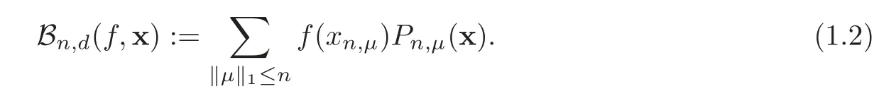
Of course,selectingtakes us back to the classical multivariate Bernstein polynomials(1.1).
The main purpose of this paper is to address the multivariate Bernstein sampling operators(1.2).Firstly,for each fixedn,we consideras random variables that take values inS,and prove a Chebyshev type error estimate.Secondly,we study the approximation orders of the sampling operators for continuous or Lebesgue integrable function,respectively.Some results in[11]are extended to the case of higher dimension.
This paper is arranged as follows.A much more general setting for uniformly distributed,modulus of continuity,and the definition of star discrepancy in simplexSare introduced in Section 2.In Section 3,we estimate the Chebyshev type error for the sampling operators(1.2).By mean of the introduced star discrepancy,we discuss the order of approximating continuous function by such operators in Section 4.Finally,theLp(1≤p<∞)convergence of the operators is studied in Section 5.
2 Notation
For a Riemann integrable functionfon the simplexS,we use the Quasi-Monto Carlo approximationwith x1,x2,···,xN∈S.An idealized model is to replace the sequence of nodes x1,···,xNby an infinite sequence of points x1,x2,···inS,such that=f(x)dx holds.The resulting condition means that the sequencex1,x2,···should be uniformly distributed in the simplexS.
A similar definition states that···are uniformly distributed in simplexSif

holds for all sub-domainFofS,whereCFis the characteristic function ofF,andλd(F)denotes the volume of sub-domainF.
For each fixedn,letP:=〉be a triangular array inS.LetJbe a family of all sub-domain ofSwith the form:

For arbitraryJ∈J,we defineA(J,P):=whereCJis the characteristic function ofJ.Thus,A(J,P)is the counting function that denotes the number of the points which belong toJ.
The concept of discrepancy is an indispensable tool in the quantitative study of uniform distribution of a finite sequence.For fixedn,we denoteN=where#denotes the number of the points which belong to the set.We now introduce a general notion of the star discrepancy of a point setP,which is given by
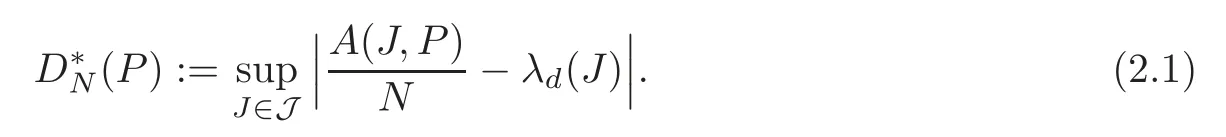
According to this definition,a triangular arrayP=〉is uniformly distributed inSif and only if=0.We refer the readers to[12]for more details about the star discrepancy.
LetC(S)denote the space of continuous function defined onSwith uniform norm

The continuity modulus of functionf∈C(S)is defined as

whereδ>0,and‖x−y‖2:=is the Euclidean distance.We say thatf∈Lip1 ifω(f,δ)=O(δ)(δ→0+).
It is easy to see that=0 and

It is clear that the Bernstein polynomials(f,x)uniformly converge tof(x)onSwhilenapproaches infinity.We are delighted to mention the following result(see[13])

which will be used in the following.
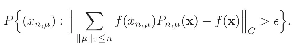
3 Chebyshev Type Error Estimate
In this section we study the following problem:Givenf∈C(S)and>0,draw points fromSindependently according to the distributionsrespectively,and estimate the probability
To get such estimate,we need estimate the following quantities.
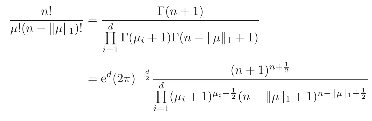
Lemma 3.1For each μ(0≤‖μ‖1≤n),we have
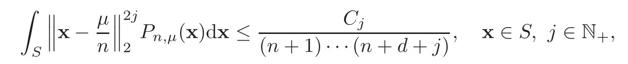
where Cjare positive constants independent of n.
ProofIt is easy to find out

where
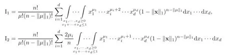
and

With Liouville formula,we can write

Similarly,

and

Note that=≤c≤1,then

We have sufficient evidence to believe that there exists a constantCjsuch that

Lemma 3.2The random variable xn,μobeys the Fμdistribution,in which for each‖μ‖1≤n,we denote by Fμthe distribution with density function:

ProofAssuming thatn∈N and x∈Sare given,we are enable to find a properδsatisfying the following conditions:D(x,δ):=⊂S,N·λd(D):=N<1.
We can find the probability of the case that the point(‖μ‖1=k)falls into the domainDisN=N·(2δ)d.
And the probability thatkselected points turn out to be in the domain×···×−δ)can be figured out by the following formula:(x−a)μ,where a={δ,···,δ}.
Further,the probability of the case that the remains appear in{y:y∈S,y≥x+a}is

Therefore,the probabilities of all these three cases mentioned above are independent of each other,and the probability that all these cases happen simultaneously is
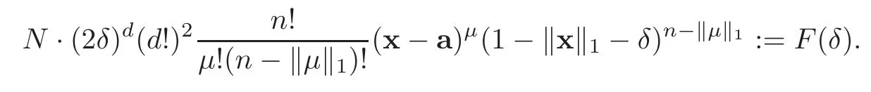
Then the density function of the random variablexn,μobeys

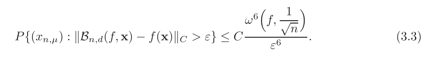
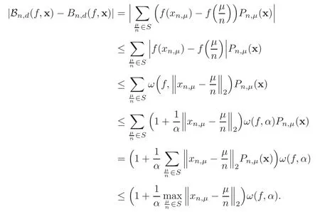
The following theorem gives a Chebyshev type error estimate of
Theorem 3.1Let ε>0and f∈C(S)be given.Suppose thatand thatare independently drawn from S according to the distributions Fμ(‖μ‖1≤n).Then there exists a positive constant C independent of n such that the following probability estimate holds:
ProofUsing(2.2)–(2.3),we have

For each fixed x∈S,we have
which implies that

Therefore,

By the assumption of the theorem,we have 3ωThus,in order that

it is necessary that

Letwe have the following inequality:

Thus,for each∈S,using Lemmas 3.1–3.2,we obtain

The proof of Theorem 3.1 is completed.
4 Approximation Order
In this section,we will discuss the approximation behavior of(f)by means of the property of.So,we first give two lemmas.
Lemma 4.1(see[14])Let x,y≥0.Then,for1≤p<∞,we have

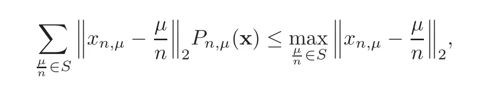
Lemma 4.2Let P=Q=〉be triangular array in S.If there holds≤ε for any given ε>0and any∈P,∈Q,then

ProofConsider any domain

Whenever≤εimplies∩S.Hence,using the inequality(4.1),we have

Similarly,

Therefore,we can deduce

Now we give an approximation behavior of(f).
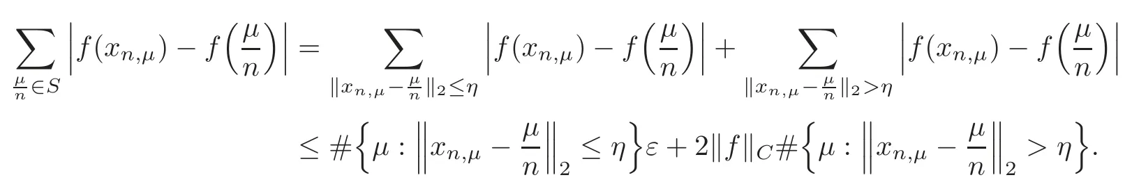
Theorem 4.1Let P=be a triangular array in S.Then we have that for any f∈C(S),

ProofForf∈C(S),according to the inequality(2.3),

It suffices to show that

Denoteα=using the property of the continuity modulus,we have
According to the inequality(4.1),we know

The proof of Theorem 4.1 is completed.
5The LpConvergence
In this section,we will study theLp(1≤p<∞)convergence for the multivariate Bernstein sampling operators.
Theorem 5.1Let P=〉be a triangular array in S.Assume that

Then for each f∈C(S),we have=0.
ProofIt suffices to show that=0.For this purpose,we find

Sincef∈C(S),for arbitraryε>0,there existsη>0 such that

Forη>0,it is easy to write

For eachε>0,from the assumptions of theorem,there existsN1>0 such that

forn≥N1.DenoteM=(x)|,thus
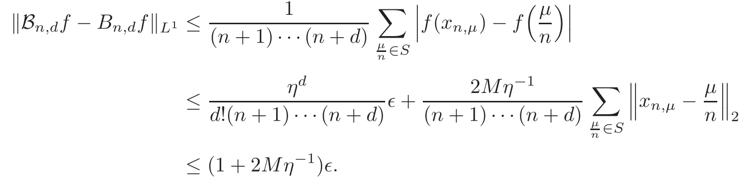
The proof of Theorem 5.1 is completed.
In order to discuss the case of 1<p<∞,we give the following lemma.
Lemma 5.1For1<p<∞,there is a constant C=Cp,dsuch that

ProofWith Liouville formula,we can write
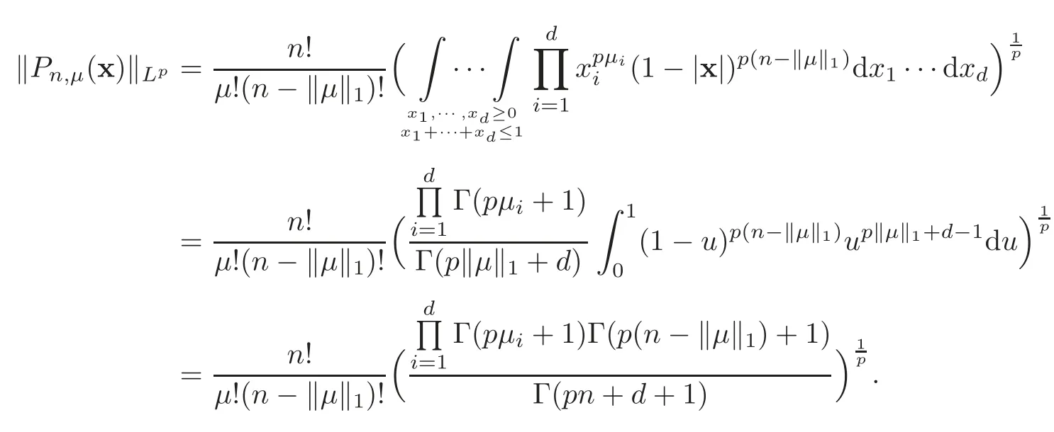
Using Sterlings formula Γ(z)∼we have
and

Thus,we can bound‖as
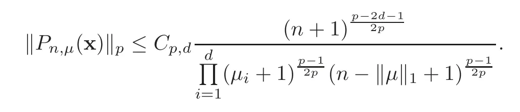
This completes the proof of Lemma 5.1.
Finally,we prove theLp(1<p<∞)convergence.
Theorem 5.2Let1<p<∞.Let P=be a triangular array in S.Let

Assume that
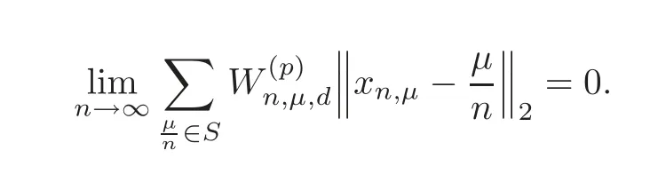
Then for each function f∈Lip1,we have=0.
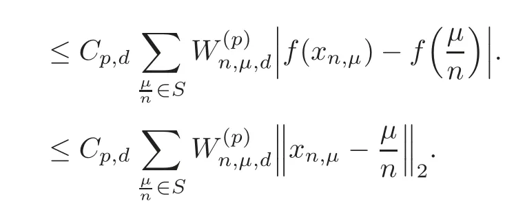
ProofIt suffices to show that=0.
Using Lemma 5.1,we have

This completes the proof of Theorem 5.2.
[1]Lorentz,G.G.,Bernstein Polynomials,Univ.Toronto Press,Toronto,1953.
[2]Ditzian,Z.,Inverse theorems for multidimensional Bernstein operators,Pacific J.Math.,121,1986,293–319.
[3]Ditzian,Z.,Best polynomial approximation and Bernstein polynomials approximation on a simplex,Indag.Math.,92,1989,243–256.
[4]Ditzian,Z.and Zhou,X.L.,Optimal approximation class for multivariate Bernstein operators,Pacific J.Math.,158,1993,93–120.
[5]Knoop,B.H.and Zhou,X.L.,The lower estimate for linear positive operators(I),Constr.Approx.,11,1995,53–66.
[6]Zhou,D.X.,Weighted approximation by multidimensional Bernstein operators,J.Approx.Theory,76,1994,403–412.
[7]Zhou,X.L.,Approximation by multivariate Bernstein operators,Results in Math.,25,1994,166–191.
[8]Zhou,X.L.,Degree of approximation associated with some elliptic operators and its applications,Approx.Theory and Its Appl.,11,1995,9–29.
[9]Cao,F.L.,Derivatives of multidimensional Bernstein operators and smoothness,J.Approx.Theory,132,2005,241–257.
[10]Ding,C.M.and Cao,F.L.,K-functionals and multivariate Bernstein polynomials,J.Approx.Theory,155,2008,125–135.
[11]Wu,Z.M.,Sun,X.P.and Ma,L.M.,Sampling scattered data with Bernstein polynomials:stochastic and deterministic error estimates,Adv.Comput.Math.,38,2013,187–205.
[12]Chazelle B.,The Discrepancy Method,Randomness and Complexity,Cambridge University Press,Cambridge,2000.
[13]Li,W.Q.,A note on the degree of approximation for Bernstein polynomials,Journal of Xiamen University(Natural Science),2,1962,119–129.
[14]Neta,B.,On 3 inequalities,Comput.Math.Appl.,6(3),1980,301–304.
 Chinese Annals of Mathematics,Series B2014年4期
- Chinese Annals of Mathematics,Series B的其它文章
- Poles of L-Functions on Quaternion Groups
- Stability of Inverse Problems for Ultrahyperbolic Equations∗
- The∂-Stabilization of a Heegaard Splitting with Distance at Least 6 is Unstabilized∗
- Monomial Base for Little q-Schur Algebra uk(2,r)at Even Roots of Unity
- Delay-Dependent Exponential Stability for Nonlinear Reaction-Diffusion Uncertain Cohen-Grossberg Neural Networks with Partially Known Transition Rates via Hardy-Poincar´e Inequality∗
- Betti Numbers of Locally Standard 2-Torus Manifolds∗