
The Periodic Solutions of a Nonhomogeneous String with Dirichlet-Neumann Condition∗
2014-06-05 03:08ChangqingTONGJingZHENG
Changqing TONG Jing ZHENG
1 Introduction
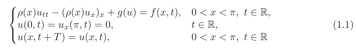
In this paper,we study the problem of time periodic solution of the nonhomogeneous string with Dirichlet-Neumann condition:
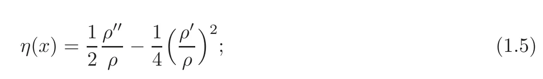
under the following hypotheses:(H1)

where
(H2)The functiong:R→R is continuous and nondecreasing,and
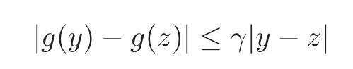
for someγ≥0.
This problem was first studied by Barbu and Pavel[2],which describes the forced vibrations of a nonhomogeneous string and the propagation of waves in nonisotropic media.After that,Ji and Li[11–12]and Rudakov[13]considered this equation with various boundary conditions,but all these papers dealed with the case when the numberω=is rational,whereTis the period of the solutions.Whenωis irrational number,the spectrum of the associated linear operator with the system(1.1)may be accumulated to zero.This is a“small divisor problem”.In order to solve the“small divisor problem”,Baldi and Berti[1]used the technique of Lyapunov-Schmidt decomposition and Nash-Moser iteration and obtained the periodic solution for Dirichlet condition.This method was widely used by many people whenρ(x)is a constant to deal irrational frequencies,even for higher spatial dimensions.About these results,one may consult Berti and Bolle[5–8],Berti,Bolle and Procesi[9].But for Dirichlet-Neumann condition,this method seems to be difficult for solving the bifurcation equation.We will use the method of Berkovits and Mawhin[4]to prove that 0 is not the accumulation point of the spectrum of the associated linear operator for some specialω.Then by adapting the method of Barbu and Pavel[2],we can obtain the existence of the periodic solution.This method avoids the tedious Nash-Moser iteration,although our result is weaker than that of Baldi and Berti in[1].
This paper is arranged as follows.In Section 2,we will prove some results about the spectrum of the linear operator associated with the system(1.1),these results are essential for our proof.In Section 3,we will use the method similar to[2]to complete the proof of our main results.In Section 4,we will list some notions and properties about continued fractions used in Section 2.
2 Some Basic Properties of the Linear Operator
Before studying the system(1.1),we need to know the properties of the spectrum of the associated linear operatorA,so we first recall some results from[2].First,some adapted complete orthonormal system of eigenfunctions

of this linear operatorAwill be needed to be taken as a basis for functions space.In order to define the operatorAand this space,some notions will be defined.
Let Ω =[0,π]×[0,T]and set

For real numberr≥1,we define

The spaceLr(Ω)is the closure ofDwith the norm‖·Suppose that the constantqsatisfies the condition=1.For functionsu∈Lp(Ω)andv∈Lq(Ω),we define

Definition 2.1A function u∈L2(Ω)is said to be a weak solution of the problem
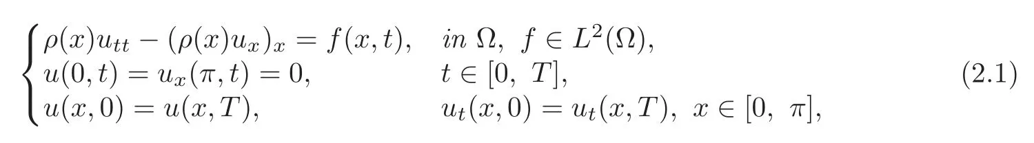
if
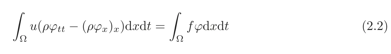
for all ϕ∈D.
Conversely,a weak solution of classC2(Ω)satisfies(2.1)in classical sense.
Set

Define:D()→L2(Ω)by

if and only if

and defineAby

Clearly,D(A)=D()contains the null function ofL2(Ω),and for eachu∈D(A)there exists precisely onef∈L2(Ω)satisfying(2.2).Therefore the operatorAdefined by(2.4)–(2.6)is a linear operatorL2(Ω)→L2(Ω)and(2.2)can be written as

where

The operatordefined by(2.4)–(2.5)is said to be the linear operator associated with(2.1).
In the following,we consider the spectrum of the operatorAon the functionsu∈L2(Ω)with the boundary condition

Using the classical method of separation of variables,we setu(x,t)=τ(t)ϕ(x)and derive thatϕmust satisfy the equation:

We denotethe eigenvalues and the eigenfunctions of the Sturm-Liouville problem(2.8).It was proved in[2]that if conditions(1.2)–(1.4)are satisfied,then there exist constants>0 such that

where

Consider the complete orthonormal system of functions

of spaceL2(Ω),where

Hence the spectrum of the linear operatorAis

The setthe following properties which is essential to the proof of our main results.
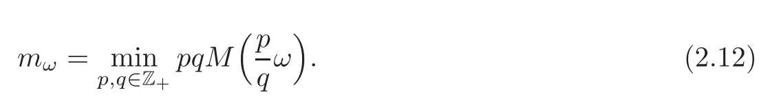
Theorem 2.1Assume that ω is irrational,and M(ω)<∞(the definition of M(ω)is in Section4).Set
If ω>2b1mω,0is not an accumulation point of
Remark 2.1Notice that it obviously has
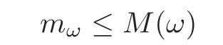
from the definition ofmω.SinceM(ω)is invariant under a translation through integers,the irrational numberωwhich satisfies the conditionsω>2b1mωexists.
ProofAssume that 0 is an accumulation point of∑Then we can find a sequenceof eigenvalues such thatσk→0 ifk→ ∞.In other words,
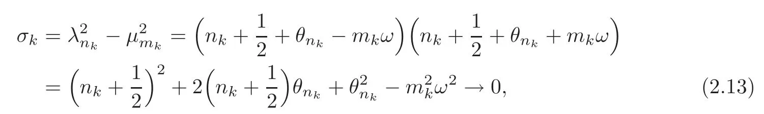
ifk→∞.Because of=0,it is equivalent to

We can write(2.14)in the form

ask→∞.We may choosemk≥0.Observing thatis bounded andnk+mkωis bounded below,then necessarily we have

and hence also

Consequently,writing(2.15)in the form
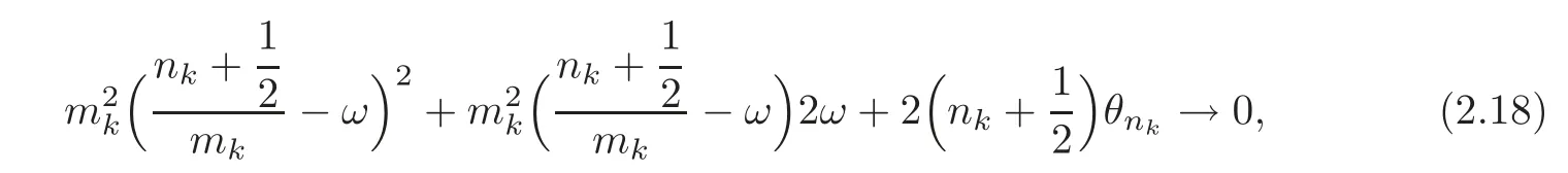
ifk→∞,we deduce that
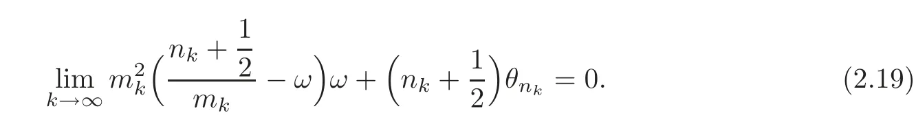
Consequently,for eachp,q∈Z+,we have
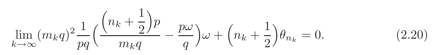
Letε>0,there existsK∈N such that

wheneverk≥K.Write above as

With this result and the definition of the functionM(ω)in Section 4,we see that

for eachε>0.Hence
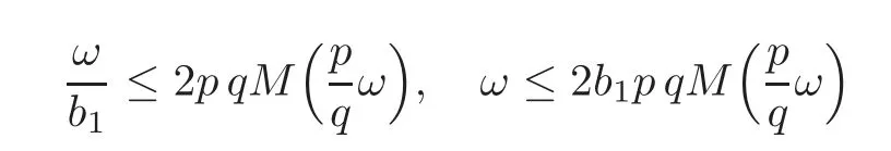
for allp,q∈Z+,and hence

a contradiction.
Now,we can prove the main result of the linear operatorA.
Proposition 2.1Let T=,and ω satisfy the condition of Theorem2.1.Then R(A)is closed in L2(Ω),A is self-adjoint and∈L(R(A),R(A)).For simplicity,we also denoteby A−1.Moreover,we have

where d=inf{|ωk|},

where α=inf{<|ωk|},

and
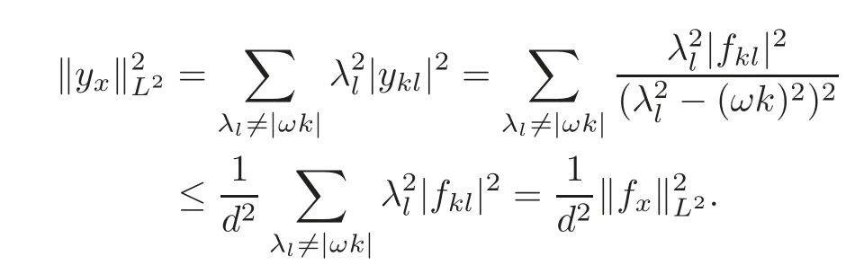
ProofWith respect to the orthonormal systemdefined by(2.8)and(2.11),the equationAy=fis equivalent to

wherey=This implies that the equationAy=fhas a solutionyonly iff∈N(A)⊥,i.e.,=0 for all(k,l)such thatλl=|ωk|.Indeed,this condition is also sufficient.For the equationAy=f,if we set

according to Theorem 2.1,0 is not an accumulation point ofSod=inf{|ωk|}>0,andis convergent.Moreover,

By(2.30),

which yields(2.24).Lety=A−1fiff∈H1(Ω)∩R(A).So its weak derivative is

whereis orthogonal inL2(0,π)and

Therefore
Similarly,it also has
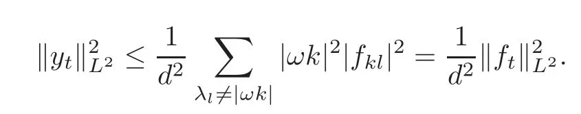
So(2.27)is proved.
In order to prove(2.26),notice that

So

whereCis a constant independent ofl.Then one has
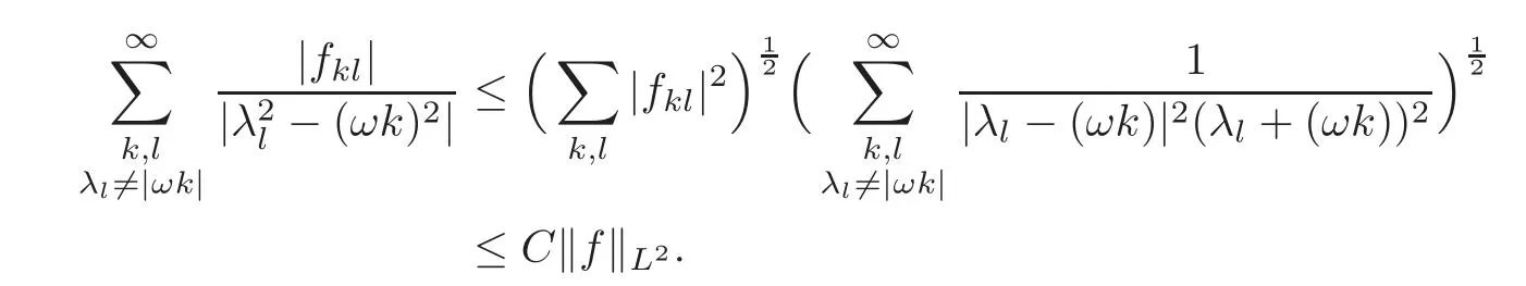
So(2.26)is proved.
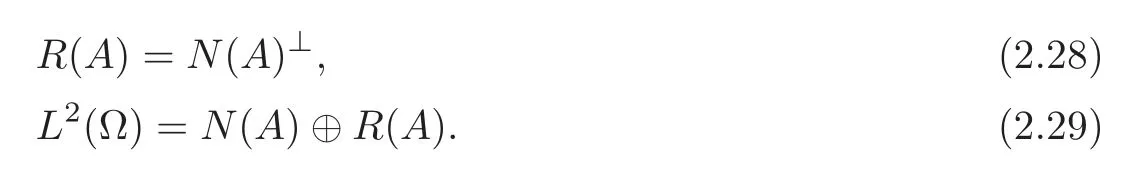
Finally,notice thatD(A)is densed inL2(Ω)andAis symmetric andR(A)=N(A)⊥.SoAis self-adjoint.
3 Proof of the Main Result
Now we begin to consider the weak periodic solution of system(1.1).Recall thatu∈L2(Ω)is a weak solution of the problem(1.1)if and only if

In order to state our main results,we give an assumption onfandgfirst.
(H3)f∈L∞(Ω)and

for someδ>0.HereP:L2(Ω)→N(A)is the projection operator onN(A).
Now we state our main result of this paper.
Theorem 3.1Assume T=,where ω is an irrational number which satisfies the condition of Theorem2.1and the hypotheses(H1)–(H3)with0<γ<α,where α=inf{|ωm|2−<|ωm|}.Then(1.1)has at least one weak solution y∈L∞(Ω).
ProofLet

In view of(H2),G:L2(Ω)→L2(Ω)is a continuous and monotone operator,i.e.,

Souis a weak solution to(1.1)in Ω if and only if

We first consider the following approximation of(3.4):

The proof will be divided into four steps.
Setp 1To prove the existence of the solution of(3.5)
LettingGε(u)=G(u)+εu,and according to the hypothesis(H2)
so

Furthermore,it obviously has

Using the idea of Brezis[10],(3.5)can be equivalently written as

Indeed,ifuis a solution of(3.5),we writeu=∈N(A),u2∈R(A),then

Letv=−Au2.Then
which shows that(3.5)and(3.9)are equivalent.
On the other hand,(3.9)is equivalent to

whereJis the indicator function ofR(A),and∂Jis the subdifferential ofJ.Taking into account that∂J(v)is the cone of the normals toR(A)atv,it follows that∂J(v)=N(A)for allv∈R(A).
Finally,(2.24)shows thatis monotone onR(A).So(3.10)can be written in the equivalent form

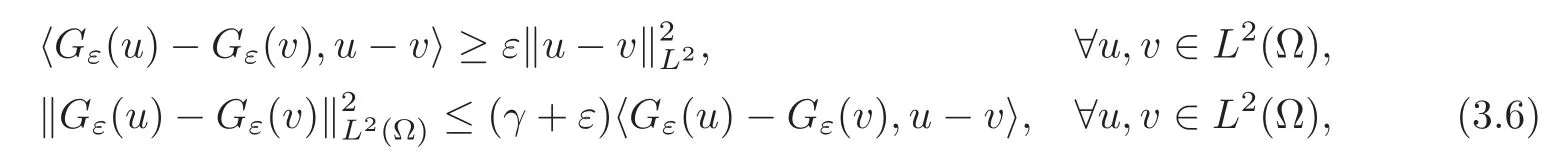
withGαv=(G+εI)−α−1v.In view of(3.11),Gαsatisfies

We now prove that(3.11)has a solutionvεfor eachε<α − γ.
On the basis of(3.12),forε<α − γ,Gαis coercive and maximal monotone inL2(Ω).
A key step now is to prove that the monotone operatorv→Aα+∂J(v)withAα==R(A)and∂J=N(A)is maximal monotone inL2(Ω),i.e.,for everyh∈L2(Ω)the equation

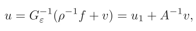
has a solutionv∈R(A).Indeed,this equation is equivalent to

which has a unique solutionv∈R(A).It follows thatAα+∂J+Gαis maximal monotone inL2(Ω).Moreover,asGαis coercive,Aα+∂J+Gαis onto.Therefore(3.11)has a solutionvε∈R(A)which is a solution of(3.10).This means that there exists∈N(A)such that

Set

Thenyε=is a solution of(3.5).
Setp 2Estimate the solutionyε
In order to estimate the solutionyεof

we note that by the assumption(H3),there existsξ=ξ(x,t)with|ξ|≤C,such that

for allδ>0 sufficiently small and|w|=1.Then the monotonicity ofgyields

withg(yε(x,t))=ρ(x,t)G(yε)(x,t).So
which impliesforwthat

for some positive constantsCandC1.
On the other hand,in view ofL2(Ω)=N(A)⊕R(A),there existsy1∈D(A)such that+Ay1andρP(ρ−1f)=g(z)=ρG(z)for somez=z(x,t)inL∞(Ω).Therefore,(3.15)can be written as

withG(z)=P(ρ−1f).Now we begin to prove that‖G()‖is bound.By(3.3),(3.17)and(2.24),we have

SubstitutingA()=G(z)−G()−into(3.18)and with the following inequality

it can be obtained
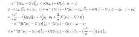

Letk=1−in(3.19),it can be obtained

So forεsmall enough,we have

By(3.21),it is easy to obtained the boundedness of|Ayε|.In fact,with(3.17)and(2.24),we have

Forεsmall enough,is bounded,henceis bounded.
Note that

With(3.16),we get

Sept 3Estimate
It is now easy to prove thatis bounded.To this goal,writewith∈N(A)andSinceis bounded inis bounded inL∞(Ω).Consequentlyis bounded inL1(Ω).So its Fourier coefficients

are bounded as|ϕn(x)|≤C,|ψm(t)|≤Cfor someCindependent ofm,n,xandt.Therefore≤≤C1.Taking into account thatN(A)is finite dimensional,it follows thatis bounded inL∞(Ω),and hence≤C.
Setp 4Taking limit asε→0
We first show that{}and{}are Cauchy sequence inL2(Ω).Set=−it is obviously that→0 inL2(Ω)asλ,ε→0.On the other hand,from(3.15)we have

Combination of(3.24),(3.3)and(2.24),it leads to

Substituting

into(3.25)and noticing thatγα−1<1,we have that|G(yε)−G(yλ)|→0 asλ,ε→0,and thereforeA(yε−yλ)is also a Cauchy sequence in(Ω).The sequence{yε}is bounded inL2(Ω),so it contains a weakly convergent subsequence(denoted it again by{yε}for simplicity).Taking into account thatG(yε)is strongly convergent inL2(Ω),it follows thatG(yε)→G(y)(strongly)inL2(Ω).Finally,it follows thaty∈D(A),Ayε →Ay,and lettingε→0,(3.15)implies(3.4).
We now can prove that actuallyyε →ystrongly inL2(Ω).Indeed,=→Aystrongly inL2(Ω).So=is also strongly convergent inL2(Ω)Theny2∈R(A).As→y−y2andN(A)is finite dimensional,it follows thatandy1∈N(A).The conclusion is thatyε→yis strongly inL2(Ω).On the other hand,yεis bounded inL∞(Ω),soy∈L∞(Ω).
4 Appendix
In this appendix,some basic properties about continued fractions will be listed and one can consult[3–4]for the proof of these results.
Letαbe real number,and puta0=[α],where[·]denotes the integer part.Then

with someα1>1 ifα>a0.Puta1=[α1]and continue the above process.Then,we obtain the continued decomposition ofα.This process does not terminate if and only ifαis an irrational number.Then we obtain the continued fraction decomposition of

and generally denote it as

wherea0,a1,a2,a3,···are integers and are called the complete quotients ofα.Generally,we denote

withpn,qnrelatively prime integers,which are the convergent ofαsuch that→ αasn→∞.
It is well known that thepn,qnare recursively defined by the following relations:

About thesepn,qn,the following theorems were proved by Ben-Naoum and Mawhin[3].
Theorem 4.1Each irrational number αcorresponds to a unique(extended)number M(α)having the following properties:
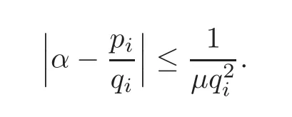
(1)For each positive number μ<M(α),there exist infinitely many pairswithsuch that

(2)If M(α)is finite,then,for each μ>M(α),there exist only finitely many pairssatisfying the inequality
The extended real numberM(α)is called the Lagrange or the Markov constant ofα.If we set

thenM(α)is an interval and Theorem 4.1 says thatM(α)=supM(α).
Theorem 4.2M(α)is finite if and only if the partial quotients sequenceof αis bounded.
Anyαwith bounded partial quotients sequenceis said to have bounded partial quotients.Borel and Bernstein have proved that the set of irrational numbers having bounded partial quotients is a dense uncountable and null subset of the real line.
Ifαis an irrational number,we need some properties on the behavior of the functionM(α)under the action of the group of transformationsTdefined by
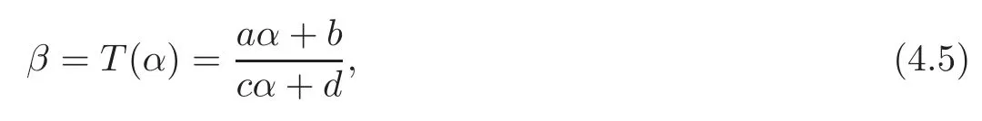
wherea,b,c,d∈Z are such thatad−bc/0.Notice that then
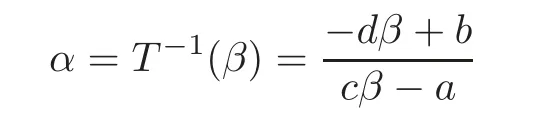
and
About this transformation,it has the following results which is proved in[4].
Theorem 4.3If β=for some a,b,c,d∈Zsuch that ad−bc/0,then

The following results are immediately from Theorem 4.3.
Corollary 4.1If β=for some a,b,c,d∈Zsuch that ad−bc/0,then β has bounded partial quotients if and only if α has bounded partial quotients.
Corollary 4.2If p and q∈Z,with p,q/0,then

The modular group is the group of transformations defined by(4.5)with|ad−bc|=1.Theorem 4.3 shows thatM(α)is invariant under the action of the modular group.In particular,whenc=0,d=1,T(α)is a translation through integers.So the Lagrange constant is invariant under translations through integers,and if{α}=α −[α],one has
AcknowledgementThe authors would like to thank the anonymous referee for their helpful comments and suggestions which lead to much improvement of the earlier version of this paper.
[1]Baldi,P.and Berti,M.,Forced vibrations of a nonhomogeneous string,SIAM J M Analysis,40,2008,382–412.
[2]Barbu,V.and Pavel,N.H.,Periodic solutions to nonlinear one-dimensional wave equation withxdependent coefficients,Trans.Amer.Math.Soc.,349,1997,2035–2048.
[3]Ben-Naoum,A.K.and Mawhin,J.,The periodic Dirichlet problem for some semilinear wave equations,J.Differential Equations,96,1992,340–354.
[4]Berkovits,J.and Mawhin,J.,Diophantine approximation,Bessel functions and radially symmetric periodic solutions of semilinear wave equations in a ball,Trans.Amer.Math.Soc.,353,2001,5041–5055.
[5]Berti,M.and Bolle,P.,Periodic solutions of nonlinear wave equations with general nonlinearities,Comm.Math.Phys.,243(2),2003,315–328.
[6]Berti,M.and Bolle,P.,Multiplicity of periodic solutions of nonlinear wave equations,Nonlinear Analysis TMA.,56(7),2004,1011–1046.
[7]Berti,M.and Bolle,P.,Cantor families of periodic solutions for completely resonant nonlinear wave equations,Duke Mathematical J.,134(2),2006,359–419.
[8]Berti,M.and Bolle,P.,Sobolev periodic solutions of nonlinear wave equations in higher spatial dimensions,Archive for Rational Mechanics and Analysis,195,2010,609–642.
[9]Berti,M.,Bolle,P.and Procesi,M.,An abstract Nash-Moser theorem with parameters and applications to PDEs,Ann.Inst.Henri Poincar Anal.,27,2010,377–399.
[10]Brzis,H.,Periodic solutions of nonlinear vibrating strings and duality principles,Bull.AMS,8,1983,409–426.
[11]Ji,S.and Li,Y.,Periodic solutions to one-dimensional wave equation withx-dependent coefficients,J.Differential Equations,229,2006,466–493.
[12]Ji,S.and Li,Y.,Time periodic solutions to one-dimensional wave equation with periodic or anti-periodic boundary conditions,Proc.Roy.Soc.Edinburgh Sect.Ser.A,137,2007,349–371.
[13]Rudakov,I.A.,Periodic solutions of a nonlinear wave equation with nonconstant coefficients,J.Differential Equations,229,2006,466–493.
 Chinese Annals of Mathematics,Series B2014年4期
- Chinese Annals of Mathematics,Series B的其它文章
- Poles of L-Functions on Quaternion Groups
- Stability of Inverse Problems for Ultrahyperbolic Equations∗
- The∂-Stabilization of a Heegaard Splitting with Distance at Least 6 is Unstabilized∗
- Monomial Base for Little q-Schur Algebra uk(2,r)at Even Roots of Unity
- Delay-Dependent Exponential Stability for Nonlinear Reaction-Diffusion Uncertain Cohen-Grossberg Neural Networks with Partially Known Transition Rates via Hardy-Poincar´e Inequality∗
- Betti Numbers of Locally Standard 2-Torus Manifolds∗