
Position Control of a Flexible Manipulator Using a New Nonlinear Self-Tuning PID Controller
2020-02-29 14:18SantanuKumarPradhanandBidyadharSubudhi
Santanu Kumar Pradhan, and Bidyadhar Subudhi,
Abstract—In this paper, a new nonlinear self-tuning PID controller (NSPIDC) is proposed to control the joint position and link deflection of a flexible-link manipulator (FLM) while it is subjected to carry different payloads. Since, payload is a critical parameter of the FLM whose variation greatly influences the controller performance. The proposed controller guarantees stability under change in payload by attenuating the non-modeled higher order dynamics using a new nonlinear autoregressive moving average with exogenous-input (NARMAX) model of the FLM. The parameters of the FLM are identified on-line using recursive least square(RLS)algorithm and using minimum variance control (MVC) laws the control parameters are updated in real-time.This proposed NSPID controller has been implemented in real-time on an experimental set-up. The joint tracking and link deflection performances of the proposed adaptive controller are compared with that of a popular direct adaptive controller(DAC). From the obtained results, it is confirmed that the proposed controller exhibits improved performance over the DAC both in terms of accurate position tracking and quick damping of link deflections when subjected to variable payloads.
I. INTRODUCTION
MAJOR challenge in manipulator control is to obtain good accuracy in positioning of the end effector.Rigidlink manipulators possess high structural stiffness. However,these manipulators are quite inefficient in terms of high speed operation and low energy consumption. Also they are unsafe to humans due to high inertia. Alternatively, flexible-link manipulators can be used in which inertia is less as a result it gives low energy consumption and high-speed operation[1]. But, while the aforesaid benefits are achieved, control of Flexible-link manipulators (FMLs) becomes difficult due to execution of following two tasks namely, rigid body position control and suppression of link-deflection [2].
When a FLM is subjected to an unknown environment due to change in payload it further affects the performance of the feedback control system [3]-[5]. Therefore, the main objective of the present work is to design an indirect selftuning PID controller with following objectives: (a) it should exhibit good joint position tracking(b)it ability to estimate online higher-order dynamics due to change in payload and (c)it should also suppress the link-deflection considerably. There have been numerous attempts in last three decades to design indirect adaptive controllers for FLMs. One of the earliest works reported in [6], [7], was on indirect adaptive controller applied to a FLM system using linear identification. However,the above adaptive controller in [6], [7] has a very limited application for large value of payloads.In[8],[9],a self-tuning controller (STC) for a two-link non-rigid manipulator was designed.But,due to the limitation in the identification method structure, there was a discrepancy during experimental validation. To overcome the complexity of neglecting dynamics of higher order for a FLM,an algebraic identification based STC was proposed in [10], which was subsequently extended for unknown loads and large payloads with an indirect controller ensuring closed-loop stability. The work in [11] was further extended for large payloads in[12].A series of simulation and experimental results established that linear identified model based STC can be used for FLM when subjected to variable loads. But, the link deflection was still a problem, first time an autoregressive moving average (ARMA) model was used to design a STC control in [13] for a single-link flexible manipulator with RLS algorithm to estimate the parameters of this model.Next,a camera was used to control the tip position in designing an adaptive controller using simple decoupled self-tuning control law comprising of the estimation of links natural frequency for a single link flexible manipulator in[14].This work was further extended by adding another sensor called accelerometer and strain gauges in [15]. Recently,there is successful effort to design intelligent PI controllers for FLMs when subjected to variable payloads [16]. Indirect adaptive controllers using a linear model fail to achieve precise real-time adaptive controller for FLM, for different payloads.Further complexity increases if the number of links increases,which gives rise to a multivariable nonlinear system. There are efforts to design nonlinear STC for nonlinear system in[17] and a multivariable STC-PID controller using minimum variance control law in [18]. To incorporate an identification technique for estimating these parameter uncertainties, the focus is to design an indirect controller using a nonlinear estimated model with help of a self-tuning controller.
The nonlinear autoregressive model is a popular nonlinear modeling paradigm since, it requires lesser number of parameters to describe nonlinear system dynamics compared to nonlinear time series representation. Hence, it involves less computational burden [19]-[26]. Also, there have been several examples where nonlinear autoregressive model based system identification is being successfully accomplished for very complex nonlinear systems, For example, in [20], a nonlinear model is used for representing nonlinear ankle dynamics systems and in [21], [22] authors used nonlinear autoregressive model for a rigid manipulator dynamics and random signal respectively.
Self-tuning controller based on estimated NARMAX model has been employed in different systems for example,Tri-Axial walking ground reaction forces in [23], a pilot-scale level plus temperature control system in [24]. Owing to the above successful implementation of NARMAX model to estimate complex nonlinear dynamics there is a motivation to design and develop a real-time implementation of a new nonlinear self-tuning controller (NSPIDC) for a Two Link Flexible Manipulator when it is subjected to handle unknown payloads[26]. To validate efficacy of the proposed NSPIDC its performances are compared with a popular direct adaptive controller[25]. The objective of our work is to design a nonlinear selftuning PID controller based on NARMAX model for a twolink FLM. The main features of the proposed control scheme are summarized as follows.
1) The control algorithm has two separate on-line tuning blocks for NARMAX parameters and the PID parameters,respectively. Stability analysis with respect to convergence of the parameter identification is also presented.
2) PID controller parameters are calculated based on the relationship between PID control and MVC laws.
The paper is organized as follows. Section II presents the dynamic model of the FLM. Section III describes direct adaptive controller for the FLM. Section IV presents the identification of FLM using NARMAX model. The proposed adaptive controller for the FLM is described in Section V.Simulation results are presented in Section VI. Experimental results are discussed in Section VII. Concluding remarks are presented in Section VIII.
II. DYNAMIC MODEL OF THE FLM
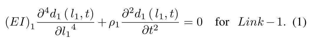
A sketch of a planar FLM is shown in Fig.1, whereτ1andτ2are the actuated torque of the Joint-1 ant Joint-2 respectively,d1(l1,t) represents the deflection along Link-1 with lengthl1andd2(l2,t) represents the deflection along Link-2 with lengthl2. The outer free end of the FLM is attached with payload mass,Mp. The dynamics of the FLM can be derived using the Lagrangian approach [5]. The total Lagrangian (L) is difference of total kinetic energy and total potential energy of the FLM system. The total kinetic energy of the can be expressed as(Total kinetic energy due to joints)+(Total kinetic energy due to links) + (Total kinetic energy due to payloadMp)in absence of gravity.The links are modeled as Euler-Bernoulli beams with deformationd1(l1,t)andd2(l2,t)for Link-1 and Link-2 respectively satisfying the link partial differential equation given as
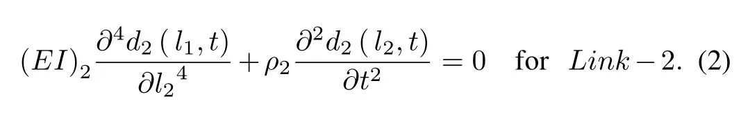
Applying boundary conditions in order to solve the above partial differential equations,the boundary conditions used are clamped-free, clamped inertia and pinned inertia. Thereafter assuming two mode of deflection for each link a finitedimensional model based on boundry conditions and assume mode method [2]. The link deflection for Link-1 and 2 are rewritten using spatial and time coordinate as
where
φ11,φ12: Mode shapes (spatial coordinate) of Link-1.
φ21,φ22: Mode shapes (spatial coordinate) of Link-2.
δ11,δ12:Modal coordinates (time coordinate)of Link-1.
δ21,δ22:Modal coordinates (time coordinate)of Link-2.
The dynamic model of the FLM is derived by using (1) to (4)for link deflection along with proper boundary conditions as described in (2). The Lagrangian-Euler dynamic equation can be written as

where
τ: Control torque applied.
q: N vector of generalized coordinates
L:KT -UT
Q: Input weighting matrix.
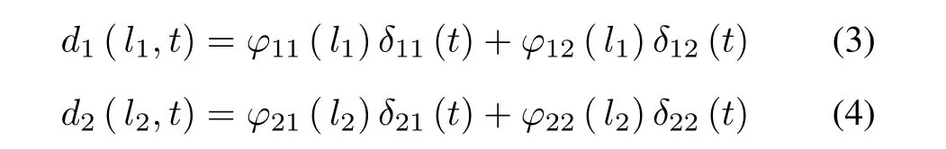
In (5), substituting the value of total kinetic energy (KT)and total potential energy(UT)of the FLM system and solving forqgeneralized coordinates, i.e., (θ1,θ2,δ11,δ12,δ21,δ22).Thus, we can write the dynamic model in matrix form as
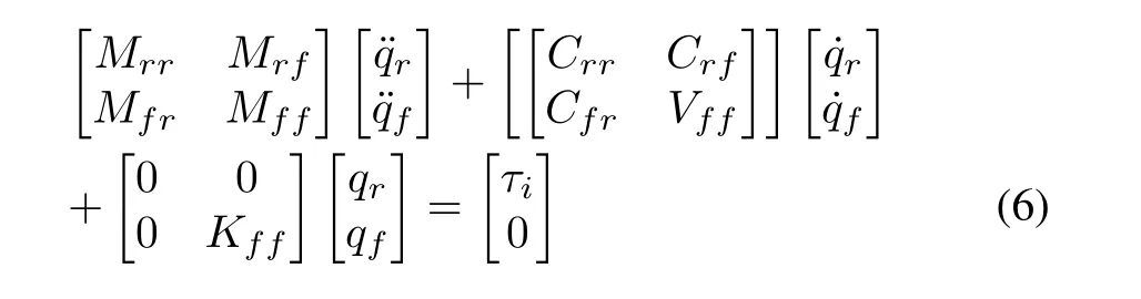
where
r,f: Rigid-mode and flexible-mode part of the FLM
M: Positive definite symmetric inertia matrix.
C: Matrix containing of Coriolis and Centrifugal forces.
Kff: Stiffness matrix =diag{kff1,kff2,kff3,kff4}.
qr:θ1,θ2are joint positions for Joint-1 and 2.
qf:δ11,δ12,δ21,δ22modal coordinates for Link-1 and 2
Equation (6) is subsequently used to design an adaptive controller.
III. DIRECT ADAPTIVE CONTROL
The design of an adaptive controller usually involves choosing a control law with tunable parameters. The objective here is to develop a Lyapunov based adaptive control scheme assuring overall system stability for a FLM.The design of this direct adaptive controller(DAC)involves in choosing a control law with tunable FLM parameters and then an adaptation law has to be developed using the closed loop error dynamics.Thus, in order to develop an adaptive controller, the dynamics of FLM in (6) is rewritten as a closed loop error dynamics using the following error signals as

and
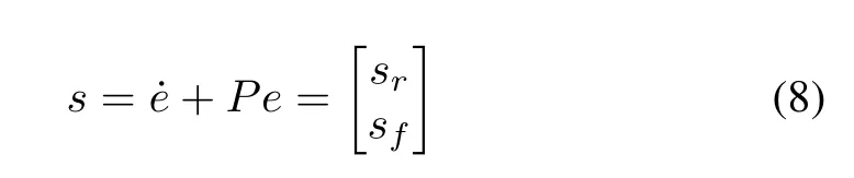
where
P: Positive definite matrix
: Desired joint positions for Joint-1 and 2.
Using error signalssr,sfdefined in(8),(6)can be rewritten as
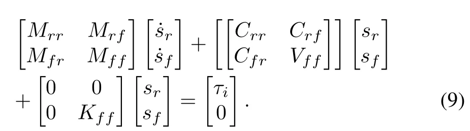
The control law is given as

where
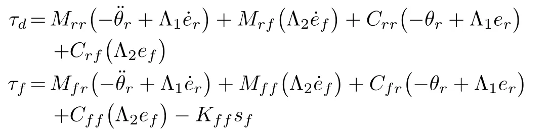
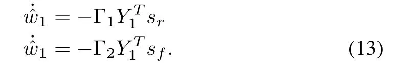
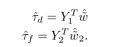
KDis a positive definite matrix.Due to change in payload,the FLM is subjected to parametric uncertainty and on account of this an adaptive control law is derived.The dynamic equations of a FLM possess the well-known linear-in-parameter property[6]. Using the linear in parameter property, we define
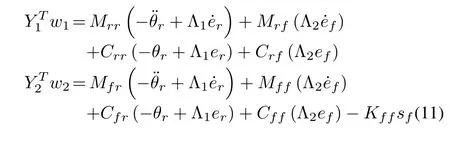
where,Y1,Y2denote the regressor matrices.w1,w2are the vectors of unknown parameters which are replaced by their respective estimates of unknown parameters as ˆw1and ˆw2control law in (10) can be rewritten as

where
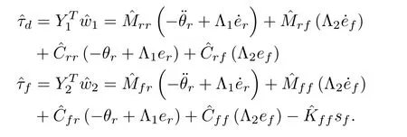
Using (13), the FLM error dynamics in(9)can be rewritten as
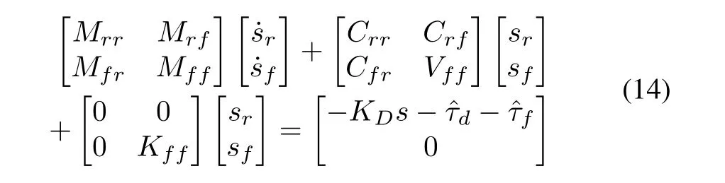
where
The structure of the control law is shown in Fig.2.Towards this end, it can be verified that the error dynamics (14) along with the adaptation law(13)are asymptotically stable by using Theorem 1.
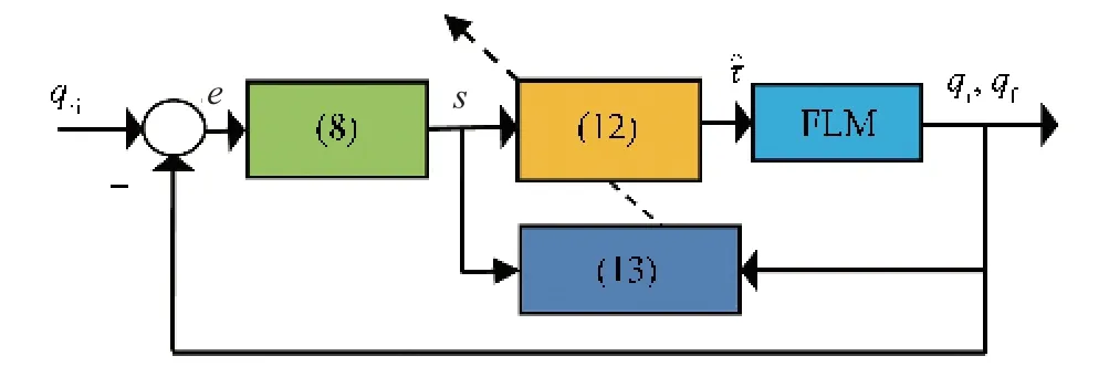
Fig.2. Structure of direct adaptive controller for FLM.
Theorem 1:The FLM dynamics described in (6) is to track a reference joint trajectory and simultaneously suppressing the link deflection when it is subjected to carry different payloads(parametric uncertainty). Then, the control law proposed in(10) and the adaptation rule (12) can achieve the above objective in finite time.
Proof:To prove this, we define a Lyapunov candidate function,V(t) as

whereMbe the mass matrix in (6) and Γ is a symmetric positive definite matrix. s is a stable first order differential equation ine. Assuming bounded initial conditions if s→0 ast →∞.Thus,differentiating(15)with respect to time leads to
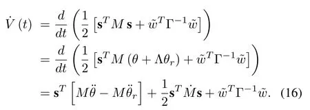
Substituting forfrom the FLM dynamics (6) and using the linear parameterizations of the FLM dynamics in (8), one obtains
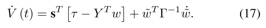
Substituting the adaptive control lawτ=-KDs-τd-τfin (17), we obtain
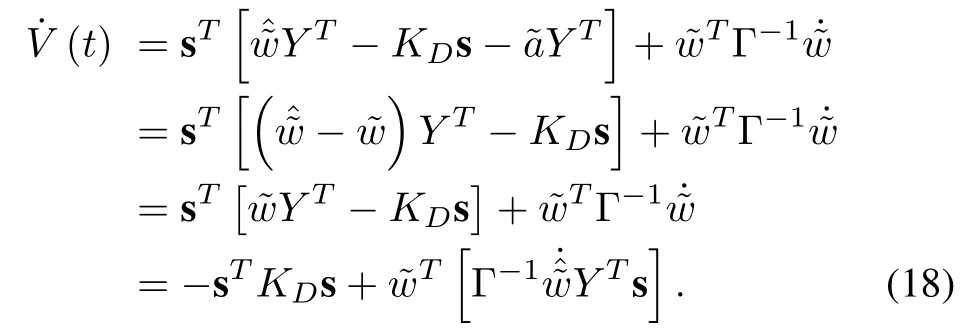
If the parameter adaptation rule iss, then
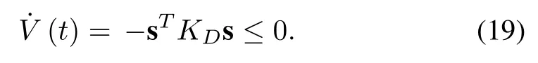
It can be seen from (17) that for some positive values ofKD,the error functions s converge to zero.
IV. IDENTIFICATION OF THE FLM USING THE PROPOSED NARMAX MODEL
冠心病心绞痛实为一种典型的临床多发病,多由于冠状动脉供血缺乏,心肌出现暂时性与急剧性缺氧、缺血所致,乃是对中老年人生命健康造成威胁的主要病症[1] 。此病较大程度影响着患者日常生活质量,严重者还有死亡风险。本文针对本院收治的冠心病心绞痛患者,采用麝香保心丸治疗,效果较好,现报道如下。
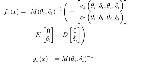

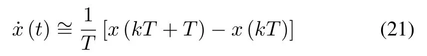
whereTis the sampling-time,x(kT) is the state vector in disctre-time.Similarly,the discrete-time representation of(20)using (21) in nonlinear form can be expressed as
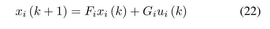
wherexi(k) denotes the joint position of theith link,ui(k)is the input to theith joint,Firepresents a multi-input multioutput (MIMO) discrete time nonlinear system matrix andGirepresent a MIMO input matrix. In order to find the inputoutput representation of the discrete-time model of the FLM let us define a new deformed output forith link as a result of link deflection defined in (3) and (4) as

In addition, a noise termχi(k) is added to (23) in order to corrupt the output of the FLM.
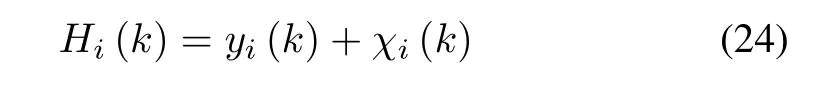
whereHi(k) is the corrupted output,yi(k) is the noise free output termed as nonlinear auto-regressive (NAR) vector andχi(k) is the additive noise input known as moving average(MA) vector andui(k) is called the exogenous input (X)vector. After collecting and compiling the terms, the overall nonlinear discrete equation is with 19 parameters (Bi(k)) for each link. The structure of the nonlinear discrete-time MIMO representation of the FLM with a tapped delay line (TDL)as a NARMAX model is shown in Fig.3. Furthermore the NARMAX model of the FLM can be rewritten using on-line estimated parameters in its regressor form as
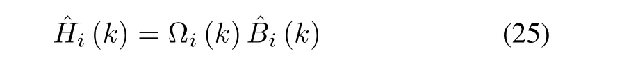
where
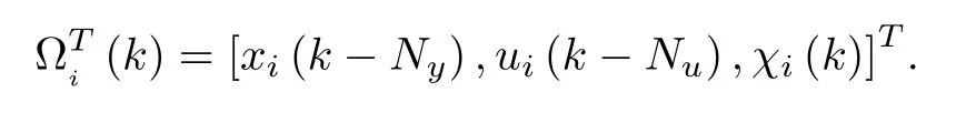
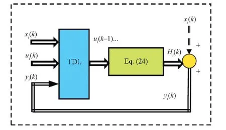
Fig.3. Structure of the (MIMO) NARMAX model of a planar FLM.
Fig.4 shows the structure for on-line recursive identification of the NARMAX model parameters. Considering the NARMAX model described in (25) some assumptions and definition are made as follows.
Assumption 1:The system ordernand relative degreeNyandNuare known a priori.
Assumption 3:The higher order of the nonlinear terms in the NARMAX model are finite.
Next a definition for bounded input bounded output(BIBO)stability for the above controller is defined.
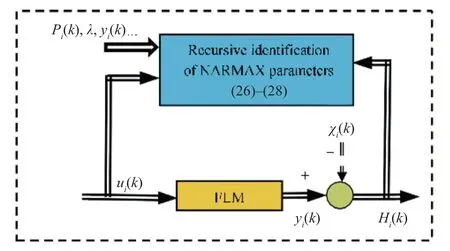
Fig.4. Structure for estimation of NARMAX parameters for FLM using RLS.
Definition 1:The system defined in (23) is BIBO stable,if and only if for every limited inputu(k) the outputy(k) is itself limited.
Mathematically:

The objective is to define a NARMAX model based multivariable self-tuning control for a FLM such that the closed-loop system is BIBO stable,while taking care the position tracking of joint position and link-deflection is improved.
Remark 1:The control inputu(k)appears with higher order nonlinear terms hence the system is non-affine.
The estimated value of parametersBi(k) of the NARMAX model (23) can be estimated using a RLS algorithm given in(26)-(29).
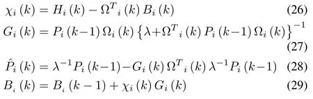
whereλis the forgetting factor andPi(k) is the covariance matrix.
V. PROPOSED NONLINEAR SELF-TUNING PID CONTROL
The proposed multivariable NSPIDC comprises of three main elements. First a representation of the nonlinear FLM dynamics in terms of multivariable difference equation NARMAX model, next an on-line recursive parameter estimation using measured input output data, and in the end a minimum variance based control law algorithm that relates the nonlinear estimated parameters to the discrete-time PID control parameters.
A. NARMAX Model Based Self-Tuning PID Controller
The input-output mapping of the FLM model represented in terms of NARMAX model in (25) NSPIDC algorithm for the FLM is described as follows. The output of NARMAX model is given by
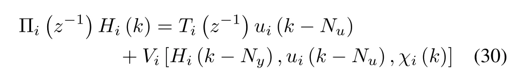
where, the polynomials Π(z-1) andTi(z-1) are linear in parameters,z-1is the backward shift operator andVi[.] is a higher order nonlinear function. In order to design a discrete time multivariable PID control law let us postulate the output of a conventional PID controller in s-domain as

The PID controller defined in (31) has the following parameters which are as follows:
KPis the proportional gain
Tiis the integral time constant
TDis the derivative time constant.
The equation can be transformed into discrete version by applying bilinear transformation,s=(2/T)[(z-1)/(z+2)],where is the sampling time period:
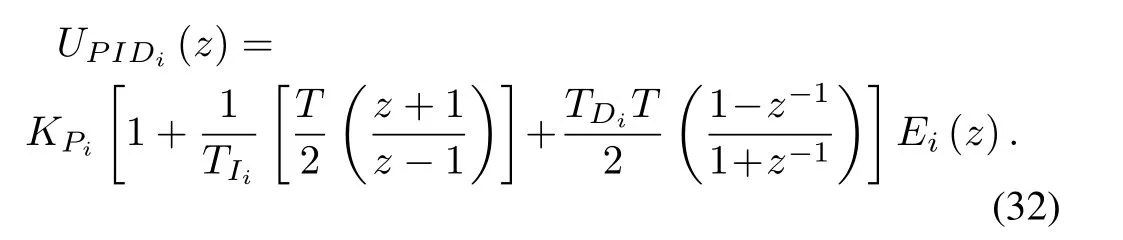
Taking inverse Z-transform and puttingT=kT0, (32) can be rewritten as
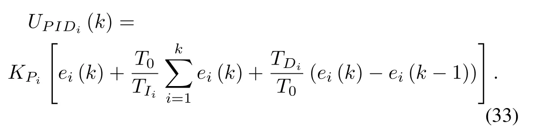
In order to apply the above equation (33) in real-time a recurrent form of the expression is used [10]
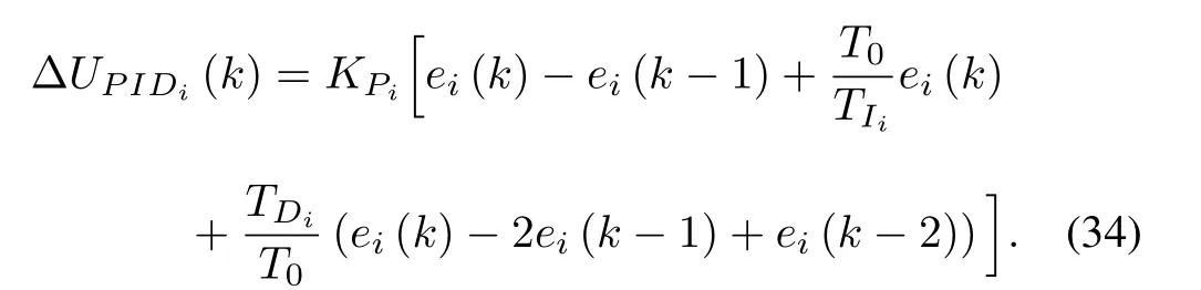
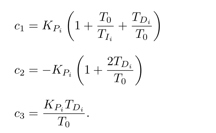
The above equation can be rewritten in terms of a polynomial

as

where
Then,using(25)we rewrite(36)in terms of the NARMAX model output as

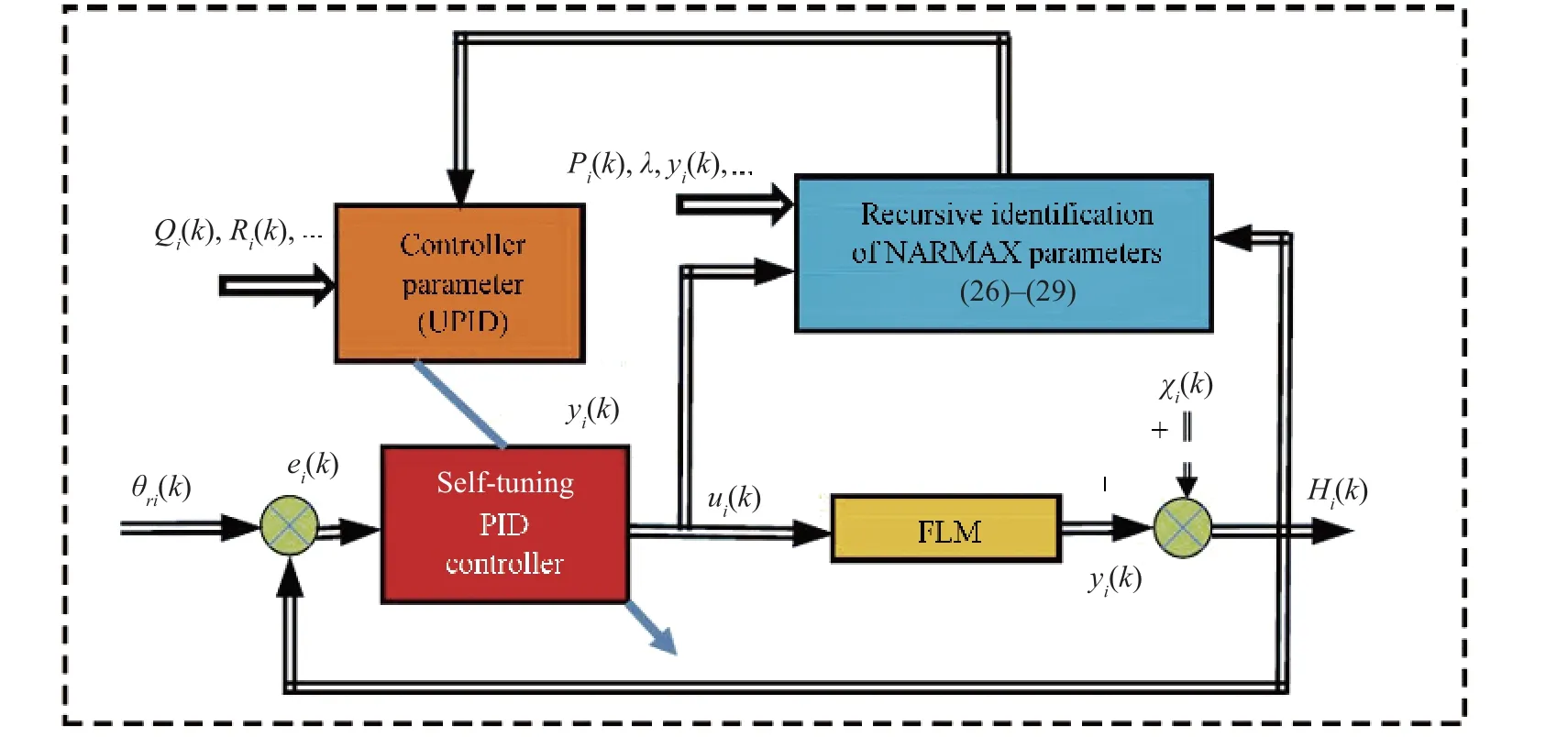
Fig.5. Block diagram of the proposed NSPIDC controller.
Equation (37) can be rewritten as
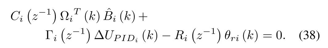
The polynomialCi(z-1)for the NSPIDC law is tuned using minimum variance control law.Fig.5 shows block diagram of the proposed NARMAX based NSPIDC for FLM,and the flow chart of the algorithm for the proposed NSPIDC is described in Fig.6.In order to tune the PID controller parameters based on the principle of minimum variance, a performance indexJis considered as follows:
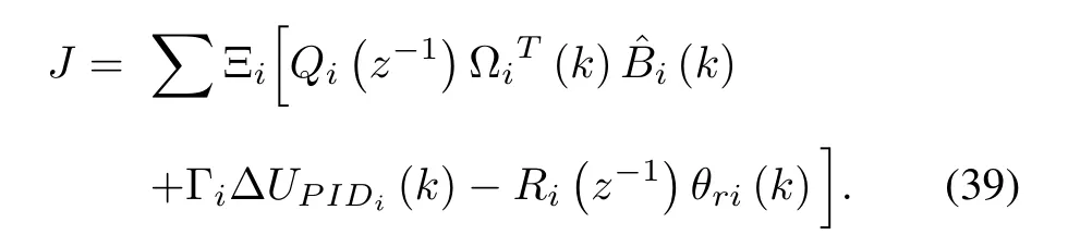
where Ξ is the expectation operator,Γiis the weighting factor with respect to the control input in(39)andQi(z-1),Ri(z-1)are user defined weighting polynomials with respect to the predicted input is the of the form

The control law minimizing the performance indexJin(39)can be obtained as
whereEi(z-1) andFi(z-1) are found out by solving the following Diophantine equation
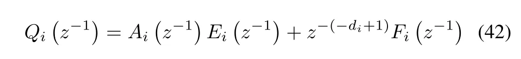
where
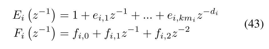
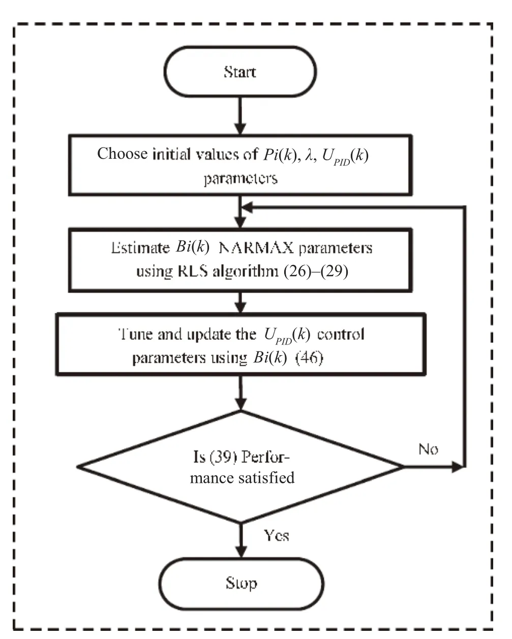
Fig.6. Flowchart of the algorithm for proposed NSPIDC.
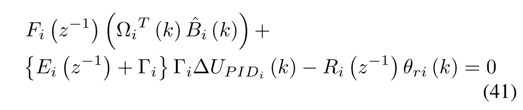
LetEi(z-1)+Γibe defined asviin (36) and now multiplying byvi(36) becomes
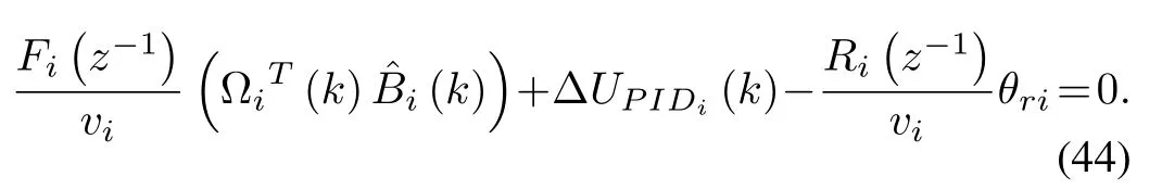
LetRi(z-1)=Fi(z-1), then (44) can be rewritten as
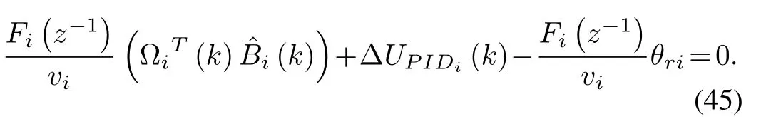
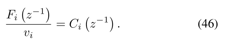
Equating (38) with (45) leads to and based on (36), (45) and (46), the PID parameterscan be calculated and updated.
B. Stability Analysis
In order to establish the BIBO stability of a nonlinear FLM system under varying payload due to proposed multivariable self-tuning control in (35), the following Theorem 2 is presented. To prove Theorem 2 for convergence of the identified parameters using the recursive identification algorithm,Lemma 1 is presented
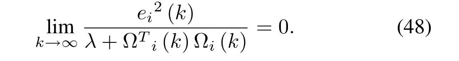
Lemma 1:The identification algorithm (26) to (29) has the following properties 1)
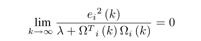
2)
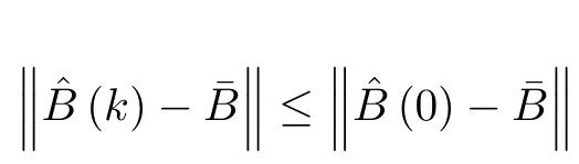
3)
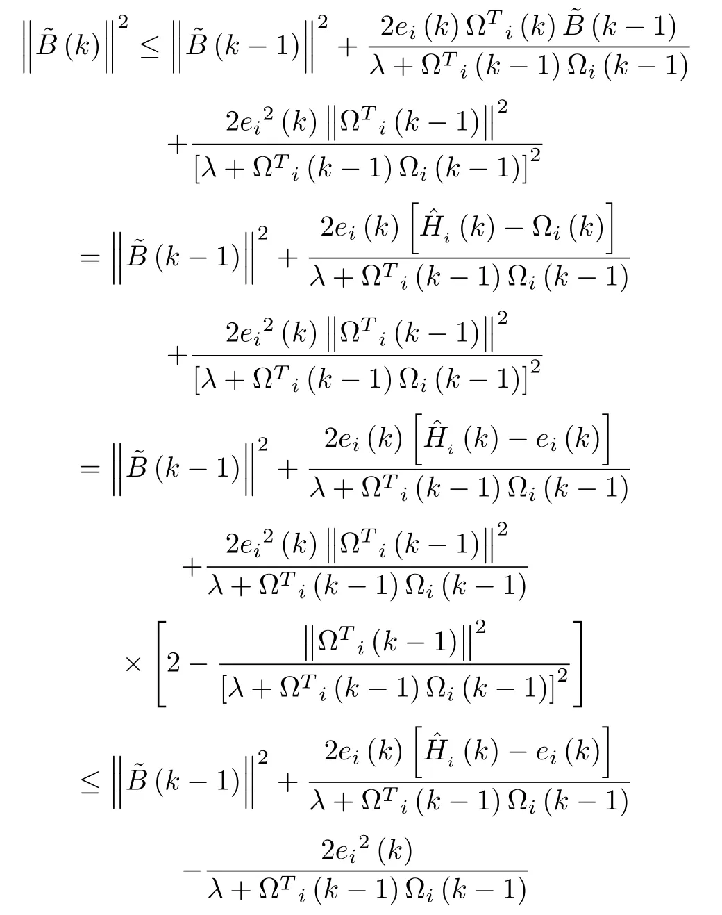
Proof: Definethen from (27) we have

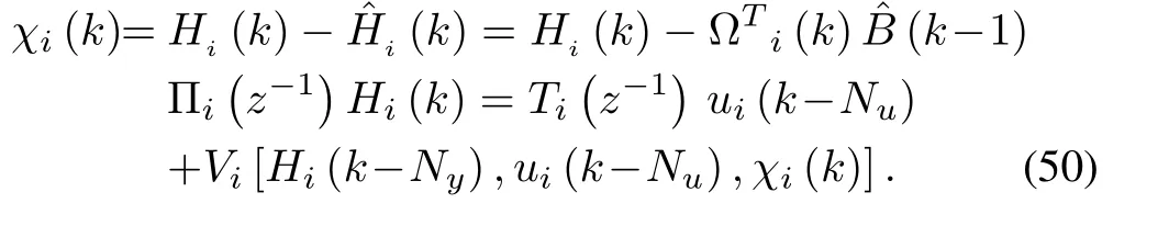
From (25) and (47) we can write that
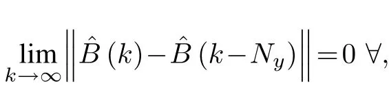
For any finite integerNy
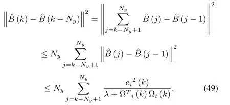
Using (49) and (50), 3) of Lemma 1 can be easily deduced.
Theorem 2:Let us consider the discrete form of the FLM system described in Theorem 1 in NARMAX representation.Also, the FLM parameters not precisely calculated while handling variable payload loads are subjected to NSPIDC such that there exist an upper bound of the parameter for the nonlinear FLM dynamic model and that the closed loop system is BIBO stable.
Proof: From (26), we have
Substituting
On multiplying both sides of (49) byEiusing matrix multiplication operator () and using (36) and (37) to the control law and unknown polynomials one obtains
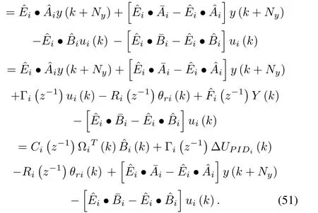
Combining (28) with (51), we further solve the above equation
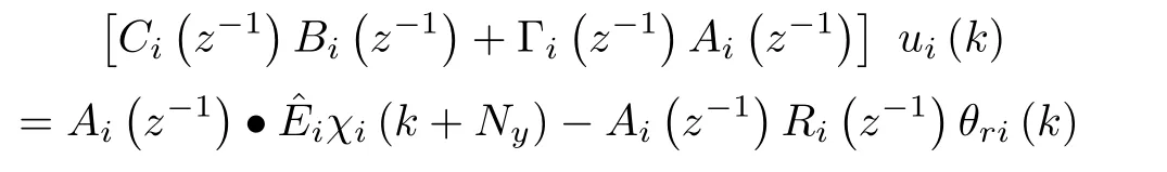
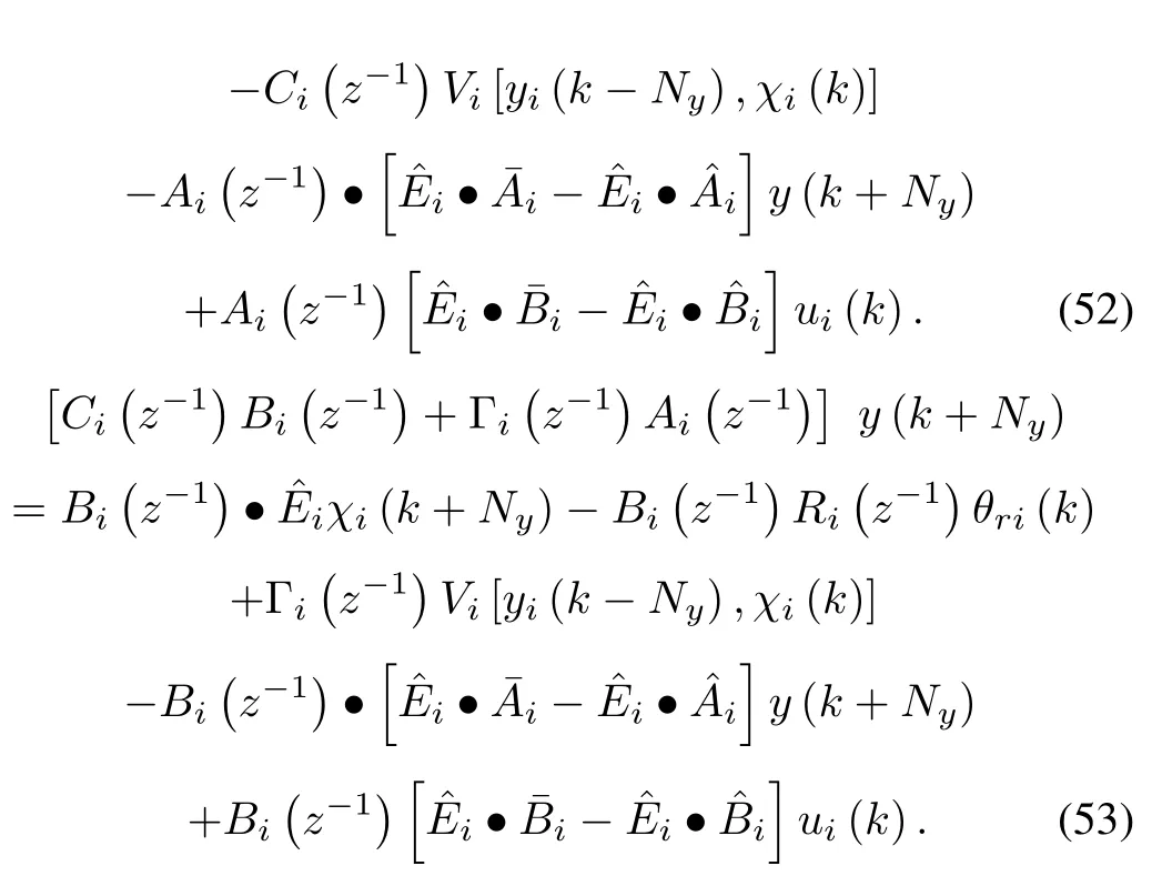
From 3) in Lemma 1, whent, the elements in square brackets on right-hand side of (52) and (53) tend to zero.Also, from 1) in Lemma 1, it may be noted that there exists a constant () positive value, for which the BIBO stability of the closed-loop system can be easily established.
VI. RESULTS AND DISCUSSIO N
The numerical simulation of the proposed NSPIDC was performed using MATLAB/SIMULINK. The proposed NSPIDC has been applied to the FLM available in Advanced Control and Robotics Research Lab., NIT, Rourkela. To validate the link trajectory tracking performances of the NSPIDC, the desired trajectory vector for two jointsθri(t) fori= 1,2 are chosen as
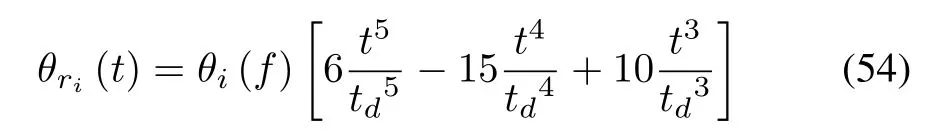
whereθri(t) = [θr1,θr2]T,θr(0) ={0,0}are the initial positions of the links andθi(f) ={π/4,π/7}are the final positions for Link-1 and Link-2,tdis the time taken to reach the finals position which is 4 s and total simulation time is set as 8 s Fig.7 shows the desired trajectory for Joint-1 and Joint-2. The physical parameters of the FLM are taken from[27].
A. Simulation Results for Controller Performance With an Initial Payload of 0.157 kg
Comparisons of performances exhibited by both the adaptive controllers(DAC and NSPIDC)while carrying a 0.157 kg payload are made in Figs.7-11. Fig.8 shows the link deflection trajectory for Link-2 carrying a nominal payload of 0.157 kg. From Fig.8 it is seen that the maximum link deflection amplitude is 0.12 m in case of DAC whereas NSPIDC yields the maximum link deflection amplitude of 0.8 m. Further, the deflections are damped out within 4 s before the link attains the final position in case of NSPIDC,whereas some oscillations in the link deflection are observed in case of DAC. Figs. 9 and 10 show the Link-2 trajectory tracking error curves. From Fig.9, it is seen that a tracking error of only 0.1 rad is achieved in case of NSPIDC for Link-1.However, the maximum tracking error is more, i.e., 0.25 rad obtained by DAC. Figs. 10 and 11 show the control torque profiles generated by NSPIDC and DAC for Joint-1 and Joint-2 respectively. The torque profiles show that the maximum torque amplitude of 10 Nm is generated in case of DAC for Joint-1 whereas 1.04 Nm is generated in case of NSPIDC.Also, the torque profile in case of Joint-2 is 11 Nm for DAC and 5Nm for NSPIDC.
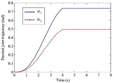
Fig.7. Desired link trajectory for Joint-1 and Joint-2
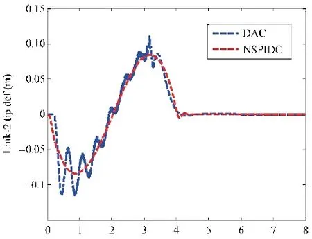
Fig.8. Link-2 deflection performances with nominal payload of 0.157 kg.

Fig.9. Link trajectory tracking errors (Link-1) with nominal payload of 0.157 kg.
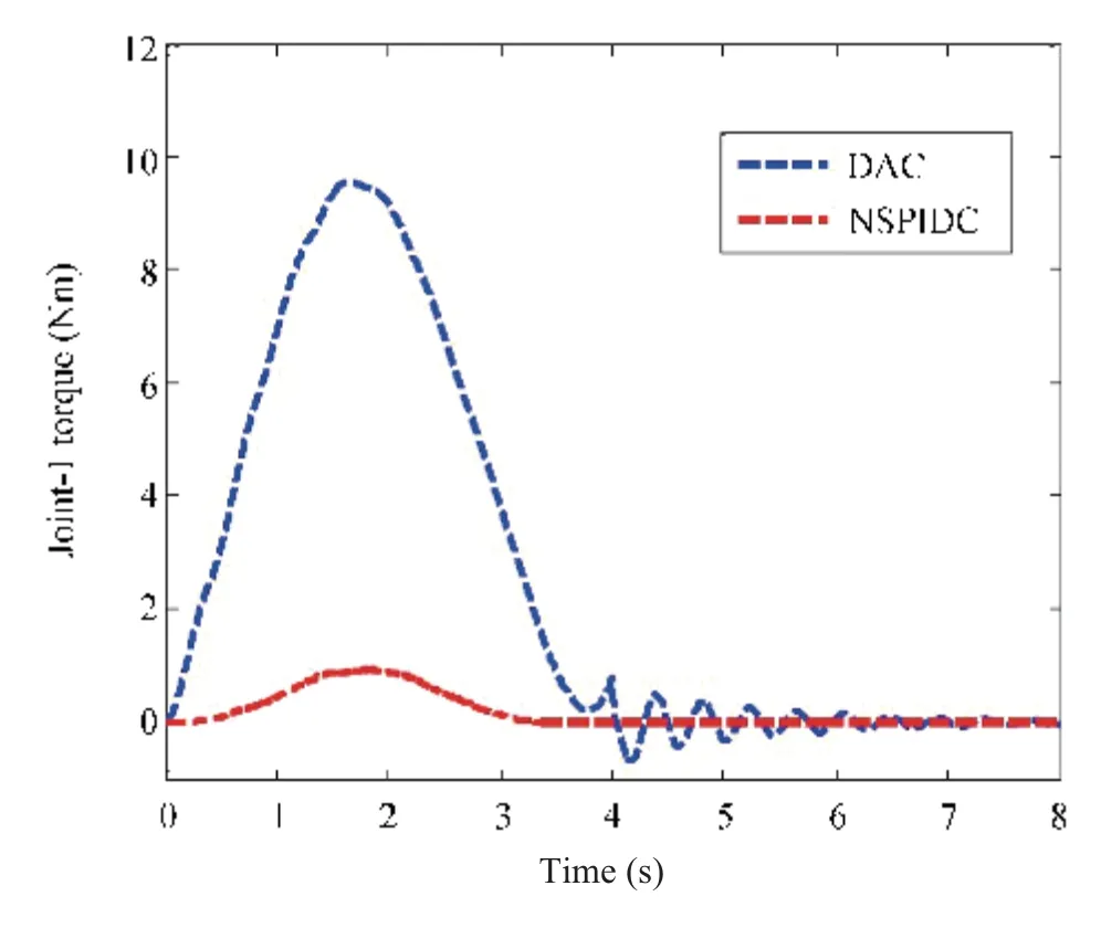
Fig.10. Torque profiles (Joint-1) with nominal payload of 0.157 kg.
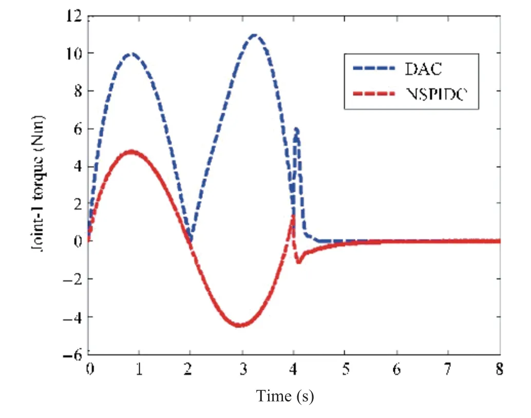
Fig.11. Torque profiles (Joint-2) with nominal payload of 0.157 kg.
B. Simulation Results for Controller Performance With an Additional Payload of 0.3 kg
In order to test the adaptive performance of the DAC compared to NSPIDC, an additional payload of 0.3 kg is now attached to the existing an initial payload of 0.157 kg.Performances of the two controllers for a 0.457 kg payload are compared in Figs.12-15. Link deflection trajectory for Link-2 is shown in Fig.12,which envisages that the maximum link deflection amplitude is 0.16 m due to DAC, whereas in case of NSPIDC, the maximum link deflection amplitude is 0.05 m. Also, damping of the Link-2 oscillations is achieved within 4 s by NSPIDC and DAC yields sustained oscillation.Fig.13 shows the link trajectory tracking error curves for Link-2. From Fig.13, it can be seen that there is a tracking error of 0.4 rad in case of DAC for Link-1. However, the tracking error is reduced to 0.2 rad in case of NSPIDC. Figs. 14 and 15 display the control torque profiles generated by NSPIDC and DAC for Joint-1 and Joint-2 respectively. From Figs. 14 and 15, it can be seen that the control input generated by the NSPIDC are 6 Nm and 8 Nm respectively which are less as compared to DAC for Link-1 and Link-2 respectively, when the desired link position is tracked. Thus, NSPIDC needs less control effort for handling an additional payload of 0.3 kg compared to the DAC.
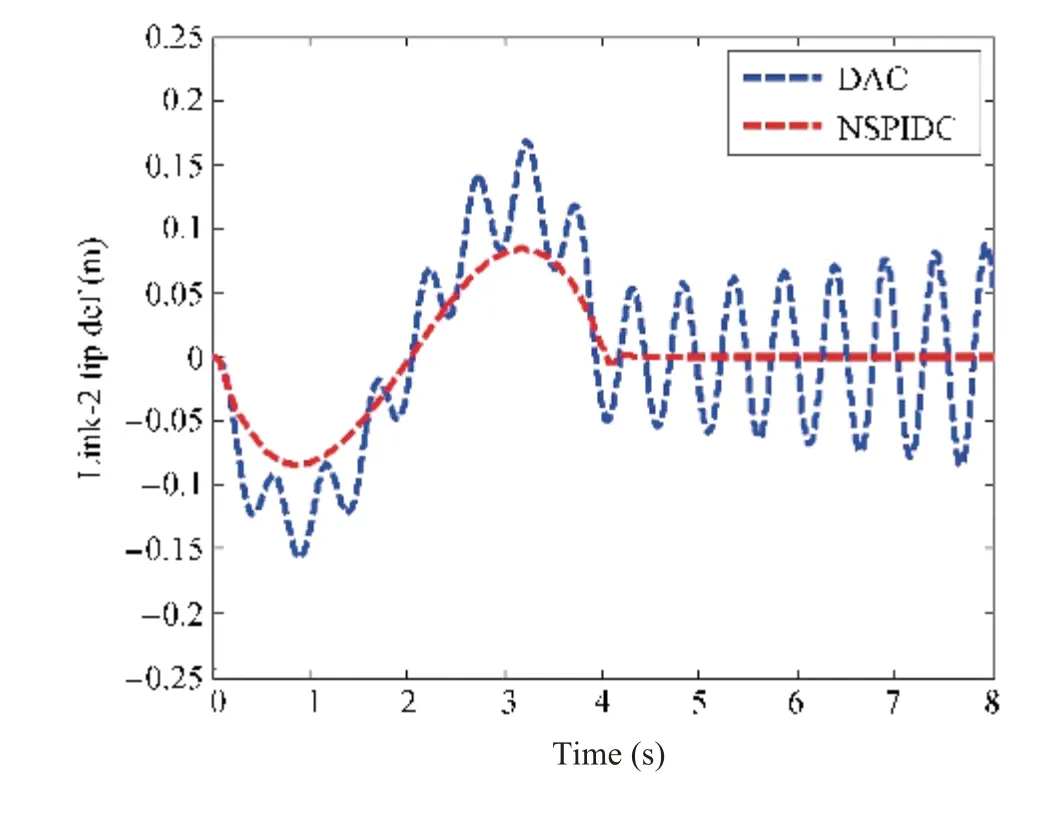
Fig.12. Link-2 deflection performances with an additional payload of 0.3 kg.
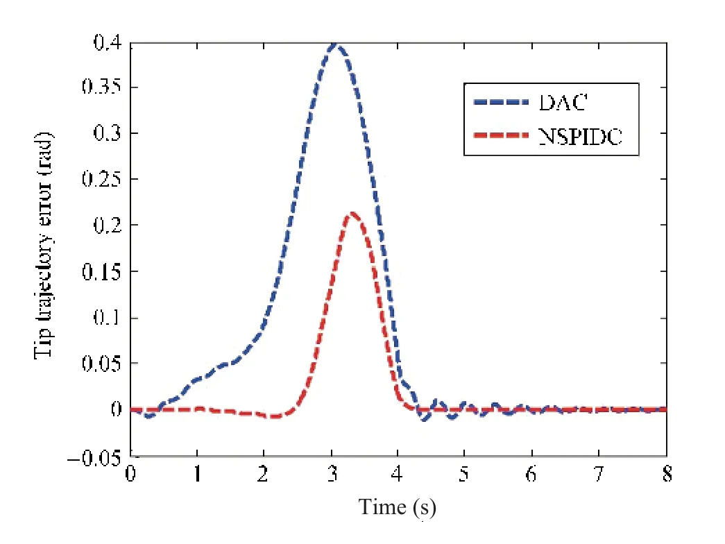
Fig.13. Link trajectory tracking errors (Link-2) with an additional payload of 0.3.
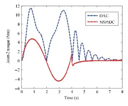
Fig.15. Torque profiles (Joint-2) with an additional payload of 0.3 kg.
C. Comparison of the Controller Performances With Respect to Position Tracking Error
The comparison of the adaptive controller with respect to position tracking error for NSPIDC and DAC under 0.157 kg of nominal payload and 0.3 kg of additional load is summarized in Table I. For comparison, performance indices such as settling time and maximum overshoot for position trajectory tracking error were chosen. From Table I it is observed that DAC yields a 35 maximum overshoot for a nominal payload and 57 for an additional load of 0.3 kg and in case of NSPIDC the maximum overshoots are 14 and 28,for nominal and additional load respectively. Tip position trajectory error settling times are as follows. It is 4 s in case of NSPIDC and corresponding settling time for DAC is 6 s for a nominal load of 0.157 kg.In case 0.457 kg payload,the settling time for NSPIDC is 4.5 s,and for DAC,it is 7.2 s.Also the comparison with respect to Power Spectral Density (PSD) is performed to check the Power/ frequency for both DAC and NSPIDC for Link-2 deflections when subjected to additional payload of 0.3 kg. The results are shown in Fig.16, a 28 dB/Hz is estimated for DAC and at the same frequency, and the PSD is 20 dB/Hz for proposed NSPIDC.
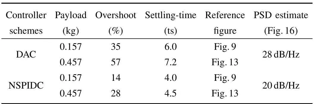
TABLE I COMPARISON OF SIMULATION RESULTS FOR THE CONTROLLERS(NSPIDC AND DAC)
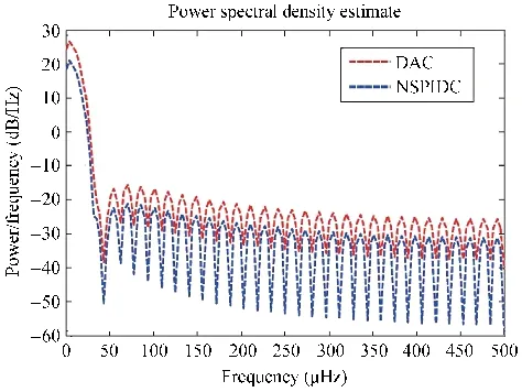
Fig.16. PSD of the Link-2 deflection with an additional payload of 0.3 kg(Fig.12).
VII. EXPERIMENTAL RESULTS
The photograph of the experimental set-up is s hown in Fig.17. The hardware and software components of the experimental set-up are described below.
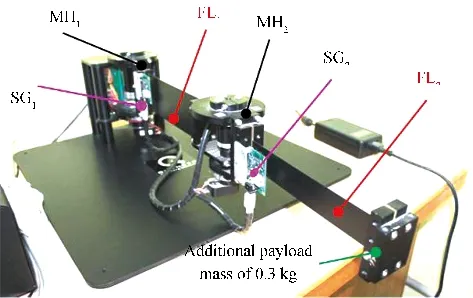
Fig.17. Photograph of the experimental set-up of the FLM.
The hardware components of the FLM constitutes a data acquisition(DAQ)board,two-channel linear current amplifier,a personal computer (PC) with Intel(R) core (TM) 2 DUO E7400 processor which operates at 2.8 GHz clock cycle., an interface board, a two-link flexible manipulator with digital optical encoders and two strain gauges at the base of each link.The FLM is provided with one pair of flexible links(FL1and FL2).This pair is made of one three-inch wide steel beam and another beam which is one-and-a-half-inch wide.
DAQ board provides two analog-to-digital(A/D)converters on board.Each A/D converter handles four channels,for a total of 8 single-ended analog inputs. Each A/D samples signals from all four channels simultaneously and holds the sampled signals while it converts the analog value to a 14-bit digital code. Each channel includes anti-aliasing filtering and input protection against electrostatic discharge (ESD) and improper connections. DAQ board has 32 channels of digital inputoutput (I/O). The channels are individually programmable as an input or an output port. All 32 channels may be read or written simultaneously. DAQ board contains four encoder chips, for position measurement each handles two channels,for a total of 8 encoder inputs. All four encoder chips can be accessed in a single 32-bit operation,and both channels can be accessed at the same time per chip. Hence, all eight encoder inputs may be processed simultaneously. There are two 32-bit general purpose counters on the DAQ board which can be used as PWM outputs with 30 ns resolution. For example,each counter can generate a 10-bit, 16 kHz, PWM signal.
The FLM is driven by two DC servo motors located at the bottom of the hub and between the joint of two links (MH1 and MH2). They are permanent magnet, brush type DC servo motors which generate a torque i =KtiIi(t), whereIi(t) is motor current forith joint whereasKt1=0.119 Nm/A andKt2=0.0234 Nm/A.Since the motors are high-speed and relatively low-torque actuators, they are coupled to the joints through a harmonic drive speed increaser with a gear ratio of 1:100 and 1:50 for Joint-1 and Joint-2 respectively. They facilitate in increasing the speed of the motors, needed to accelerate the links. The optical incremental encoder is attached to the DC servo motor making the hub position i digitally available.This digital signal is decoded through an integrated circuitry on the interface board feed-back. In addition to 32 digital I/O channels, the DAQ board has four additional channels for special two digital inputs and two digital outputs. One strain gauge sensor to measure the bending deformation of the link is mounted at the clamped base of each flexible link (SG1 and SG2). Each strain gauge sensor is connected to its own signal conditioning and amplifier board. The amplifier board is equipped with two 20-turn potentiometers.
The interfacing of software signals for the FLM set-up works on MS Windows operating system with the MATLAB/SIMULINK 2007a software.There is a provision of realtime target logic code builder to interface the SIMULINK model. The MATLAB code for controller is built up in the real-time set up by using the real-time target logic code in C language. The PC program written in MATLAB uses C language as a user interface program for the host PC which starts up the DAQ board to interact with it and with the user.
A. Experimental Results for Controller Performance With an Initial Payload of 0.157 kg
Figs.18-21 compare the experimental results obtained with DAC and NSPIDC when the manipulator is subjected to carry an initial payload of 0.157 kg. Fig.18 shows the link deflection trajectories for Link-2 carrying a nominal payload of 0.157 kg. From Fig.18, it is observed that Link-2 exhibits a link deflection of 0.3 m in case of DAC but less deflection is observed for NSPIDC i.e. the deflection has been reduced to 0.15 m. Fig.19 shows the tip trajectory tracking error curve.From Fig.18 it is seen that there is a tracking error of 0.18 rad in case of DAC. However, the tracking error in case of NSPIDC is 0.12 rad.
Figs. 20 and 21 show the control torque profiles generated by NSPIDC and DAC for Joint-1 and Joint-2 respectively.The maximum value of control torque is 0.5 Nm and reduces to almost zero after 2 s in case of NSPIDC, whereas for DAC,the maximum value is 9 Nm and it remains at 4 Nm till the link attains its final position.The torque profiles for Joint-2,in case of DAC attains 12 Nm and reduces to almost zero after 4 s whereas for NSPIDC the maximum input control torque is less i.e. 0.05 Nm initially, then rises to 0.2 Nm and it is maintained at 0.1 Nm till the link attains its final position.
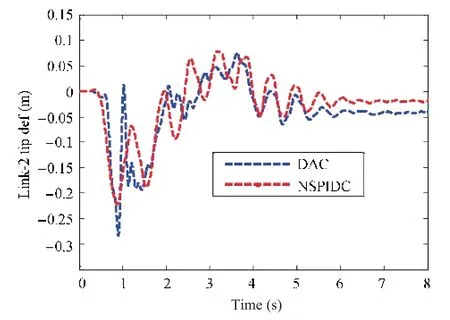
Fig.18. Link-2 deflection performances with nominal payload of 0.157 kg.
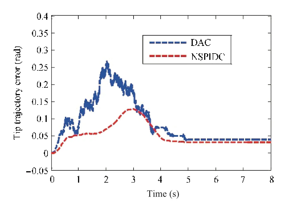
Fig.19. Link trajectory tracking errors (Link-2) with nominal payload of 0.157 kg.
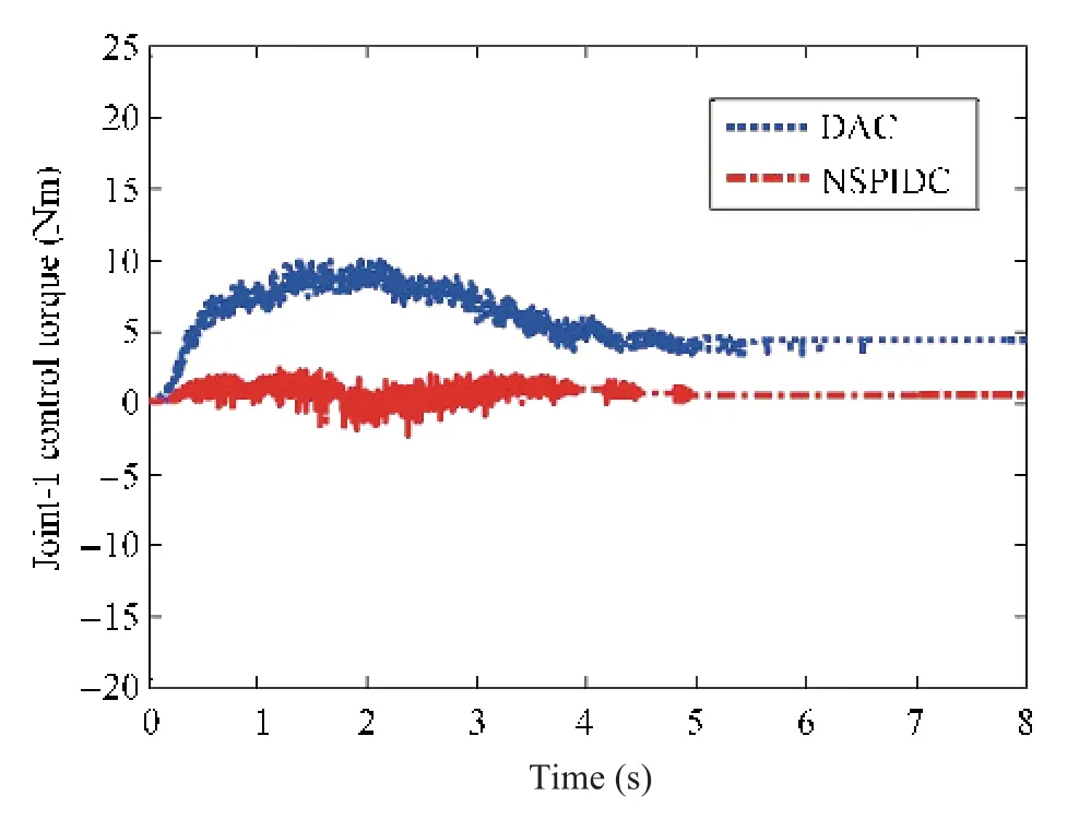
Fig.20. Torque profiles (Joint-1) with nominal payload of 0.157 kg.
B. Experimental Results for Controller Performance With an Additional Payload of 0.3 kg
To verify the adaptiveness of the controllers for handling a new payload of 0.3 kg, performances of DAC and NSPIDC for 0.457 kg payload were compared in Figs.22-25. Fig.22 shows the tip deflection profile of the Link-1.Fig.22 envisages that DAC yields a maximum deflection up to 0.4 m and damps out oscillation at 6 s whereas NSPIDC yields less deflection i.e. 0.2 m and settles at 5 s. Fig.23 shows the tip trajectory tracking error curves.From the figure,it is observed that,DAC needs less control input for handling a payload of 0.457 kg compared to the NSPIDC. From Fig.23, it is seen that there is a tracking error of 0.1 rad in case of NSPIDC for Link-1,however,the tracking error in case of DAC is 1.5 rad.Figs.24 and 25 show the control torque profiles generated by NSPIDC and DAC for Joint-1 and Joint-2 respectively. From Figs. 24 and 25, it is seen that the control input generated by the DAC is almost at 5 Nm whereas in case of NSPIDC the input torque is almost zero after 4 s.
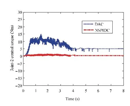
Fig.21. Torque profiles (Joint-2) with nominal payload of 0.157 kg.

Fig.25. Torque profiles (Joint-2) with an additional payload of 0.3 kg.
C. Comparison of the Controller Performances With Respect to Position Tracking Error
The comparison of the adaptive controller with respect to position tracking error for NSPIDC and DAC with 0.157 kg of nominal payload and 0.3 kg of additional load is summarized in Table II. The comparison of performance indices such as settling time and maximum overshoot for position trajectory tracking error were chosen. From Table II, it is observed that DAC yields a 32 maximum overshoot under nominal payload and 50 for additional load of 0.3 kg and in case of NSPIDC,the maximum overshoots are 17 and 28,for nominal and additional load respectively. Tip position trajectory error settling times are as follows. It is 4 s in case of NSPIDC and corresponding settling time for DAC is 5 s for a nominal load of 0.157 kg. In case 0.457 kg payload, the settling time for NSPIDC is 5 s, and for DAC the value is 6 s. Also the comparison with respect to PSD is performed to check the Power/ frequency for both DAC and NSPIC for Link-2 deflections when subjected to additional payload of 0.3 kg.The results are shown in Fig. 26. 29 dB/Hz is estimated for DAC and at the same frequency, the PSD is 26 dB/Hz for the proposed NSPIDC.
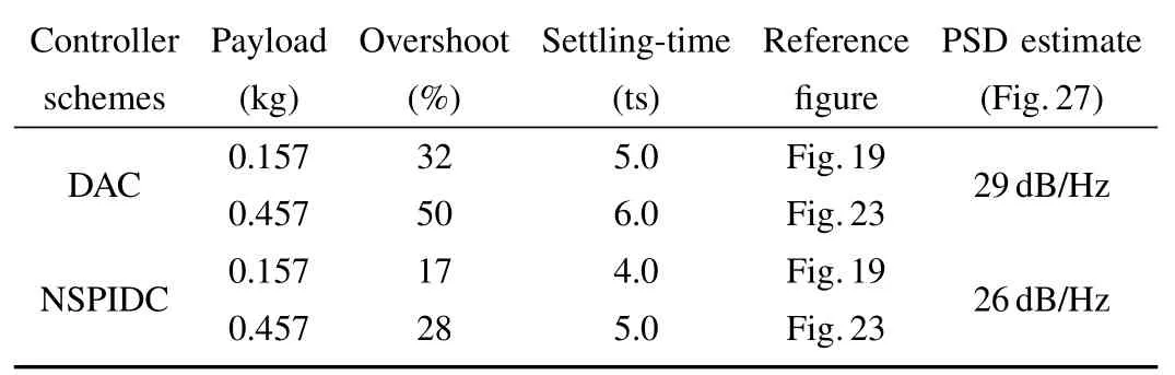
TABLE II COMPARISON OF EXPERIMENTAL RESULTS FOR THE CONTROLLERS(NSPIDC AND DAC)
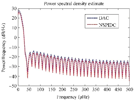
Fig.26. PSD of the Link-2 deflection with an additional payload of 0.3 kg(Fig.22).
D. Comparison of the Controller Performances With Respect to Simulation and Experimental Results
The results obtained from both experiment and simulation in terms of both time domain specification as well as frequency spectrum analysis are summarized in Tables I and II. The results show that in terms of maximum overshoot and settling time,the simulation results match with the experimental results with an error margin of 2-5. However, in terms of frequency spectrum analysis the simulation and experimental results for link-deflection show an error of around 5.Therefore,it can be said that the estimated nonlinear NARMAX model identifies the complex nonlinear dynamics of FLM when subjected to variable payload.
VIII. CONCLUSION
The paper has presented a new self-tuning multivariable PID controller to control joint trajectory and link deflection of a two-link flexible manipulator while handling variable payloads based on NARMAX model. The proposed NSPIDC has been applied successfully to a flexible robot set-up in the laboratory.From the simulation and experimental results it is established that the proposed NSPIDC generates appropriate adaptive torque when the manipulator is asked to handle additional payload.The reason is that,in case of NSPIDC,parameters are adapted due to change in payload by directly estimating the NARMAX model parameters on-line using a RLS algorithm whereas in case of DAC parameters adaptations are based on Lyapunov direct method.
猜你喜欢
医院管理论坛(2022年7期)2022-10-14
现代临床医学(2021年3期)2021-07-16
现代临床医学(2021年1期)2021-01-26
天津中医药(2020年10期)2020-12-10
中外医疗(2020年5期)2020-06-11
天津中医药(2020年5期)2020-06-01
大经贸(2020年1期)2020-04-07
农家科技下旬刊(2019年3期)2019-07-08
作文周刊(高考版)(2019年3期)2019-04-17
天然产物研究与开发(2018年8期)2018-09-10
 IEEE/CAA Journal of Automatica Sinica2020年1期
- IEEE/CAA Journal of Automatica Sinica的其它文章
- Networked Control Systems:A Survey of Trends and Techniques
- Big Data Analytics in Telecommunications: Literature Review and Architecture Recommendations
- A Stable Analytical Solution Method for Car-Like Robot Trajectory Tracking and Optimization
- A New Robust Adaptive Neural Network Backstepping Control for Single Machine Infinite Power System With TCSC
- Algorithms to Compute the Largest Invariant Set Contained in an Algebraic Set for Continuous-Time and Discrete-Time Nonlinear Systems
- Asynchronous Observer Design for Switched Linear Systems: A Tube-Based Approach