Improved Analysis of PINNs: Alleviate the CoD for Compositional Solutions

Yuling Jiao, Xiliang Lu, Jerry Zhijian Yang,Cheng Yuan and Pingwen Zhang,3,*

1 School of Mathematics and Statistics, Wuhan University, Wuhan,Hubei 430072, China

2Hubei Key Laboratory of Computational Science,Wuhan University,Wuhan,Hubei 430072, China

3School of Mathematical Sciences, Peking University, Beijing 100871,China

Abstract. In this paper, we present an improved analysis of the Physics Informed Neural Networks(PINNs)method for solving second-order elliptic equations. By assuming an intrinsic sparse structure in the underlying solution,we provide a convergence rate analysis that can overcome the curse of dimensionality(CoD).Specifically, using some approximation theory in Sobolev space together with the multivariate Faa di Bruno formula, we first derive the approximation error for composition functions with a small degree of freedom in each compositional layer. Furthermore, by integrating several results on the statistical error of neural networks, we obtain a refined convergence rate analysis for PINNs in solving elliptic equations with compositional solutions. We also demonstrate the benefits of the intrinsic sparse structure with two simple numerical examples.

Key words: Composition function, deep neural network, approximation.

1 Introduction

With recent success of neural networks in many areas of science computation [1–6], solving partial different equations(PDEs) with deep learning methods has been widely studied, e.g., the Physics-Informed Neural Networks (PINNs) [7], the Deep Ritz Method (DRM) [8] and the Weak Adversarial Neural Networks (WAN) [9].While both DRM and WAN use the weak form of PDEs, PINNs solves PDEs by a direct minimization of the square residuals in strong form,which makes the method more flexible and easier to formulate for general problems. Unlike classical function approximation strategies like polynomial approximation or Fourier transforms,deep neural networks turns out to be an easy-to-implement tool which shows impressive expressive power in dealing with several high-dimensional problems, such as solving the Kolmogorov PDEs [10].

On the other hand, several theoretical works on the approximation theory of DNN and the convergence rage of PINNs have also been done. For instance, based on the localized polynomial approximation Yarotsky establishes an upper and lower bound for DNN with ReLU as an activation function [11]; Shen et al. study the approximation error for smooth functions[12]and Hölder continuous functions[13],resulting in a non-asymptotic estimation characterized by width and depth of the DNN. More recently, in the context of solving PDEs with deep learning method,the approximation theory of DNN has also been generalized to the Sobolev space.In [14] Gühring et al. extend Yarotsky’s proof to the higher-order Sobolev space,with the help of approximate partition of unity and averaged Taylor polynomials.Hon et al. also obtain a simultaneous approximation result in Sobolev space for smooth functions [15], with a similar construction proof as in [12]. In the meanwhile, in [16,17] the authors provide rigorous convergence analysis for PINNs and DRM by simultaneously controlling the approximation error and the generalization error of deep neural networks. According to these results, however, the curse of dimensionality (CoD) still exists in general situation if no additional assumption is made on the targeted function itself. In the past years, one such function space is the Barron classes. Inspired by the original work by Barron[18],E et al. studied the approximation ability of two-layer neural networks for the Barron space and residual neural network for the flow-induced function spaces [19], of which the convergence rate is independent of the dimensionality. Furthermore,Lu et al.[20]give an analysis of the DRM method for a two-layer neural network space, which also shows the CoD can be avoided if the solution is in the Barron space. More recently,they study some sufficient conditions for the equations to admit such a solution [21,22].

In this work, we present an improved analysis for PINNs with compositional solutions. By assuming a sparse structure in each composition layer, we show that the total compositional function in high dimensional space owns a low-dimensional property, in the sense that it can be approximated by DNN with a convergence rate only dependent on the intrinsic low dimension. In practice, such a composition function is commonly used,such as the derivative of potential function(atom force)in Molecular Dynamics (MD) simulation with the embedded-atom potential, which is a composition function in high-dimensional space while possessing an intrinsic low-dimensional structure due to the cutoffeffect in the pairwise potential and embedding energy [23]. Furthermore, as stated by Kang and Gong [24], if we use a simple forward Euler method to solve the MD system, the numerical solution at a given time can be regarded as a compositional function of the initial position,in which each compositional layer is also an intrinsic low-dimensional function. A similar set up has also been considered by Dahmen in[25],in which the author proves that the solution of a linear parametric transport equation has a compositional sparse structure if the convection field does so. While Dahmen studies the approximation effectiveness withL∞norm of ReLU DNN by restricting to a function space with quantifiable compositional dimension sparsity,we would focus on the approximation theory ofReLUsDNN for compositional function withCsnorm. Furthermore,by integrating some existing work on the statistical error in solving PDEs with DNN [16,17,26,27], we would use the approximation result to obtain a convergence rate analysis for the PINNs method in solving elliptic equation with composition function as the solution. In summary, our main contributions are as follows:

·We obtain an approximation result for the composition functions,see Theorem 4.3. Formally,for a compositional functionhq◦···◦h0in whichhi(x)∈Cs([0,1]d)is at-variate function,there exists aReLUsfunctionwith widthO()and depthq(「log2+2)-qsuch that

·As an application, we prove that under some conditions (see Theorem 3.1),if we set theReLUsfunction space with widthO() and depthq(「log2+2)-q,and let the sample size of inner pointsXkand boundary pointsYkbeing

the expected error of PINNs solutionscan be bounded as

The rest of this paper is organized as follows. In Section 2, we briefly introduce some notations of compositional functions, deep neural networks and norm spaces.Next, in Section 3, we present the main theorem on the convergence rate of PINNs for elliptic equation with compositional solutions. In Section 4,we provide the proof of the approximation error of compositional functions. Two illustrative numerical examples will be given in Section 5, followed by the final conclusion in Section 6.

2 Preliminaries

As a beginning, we introduce some notations on the neural networks and normed space. Letf0denote the target function (or called regression function) with similar set up as in[28]. We assumef0is a composition of a series of functionshi,i=0,...,q,i.e.,

wherehi:[0,1]di→[0,1]di+1. For eachhi,denote bythe components ofhiand lettibe the maximal number of variables on which each ofhijdepends.Note thatti≤diand eachhijis ati-variate function forj=1,...,di+1.

As to the approximation space(hypothesis class), we set the function classFto beFD,W,U,S,B, a class of feed forward neural networksφθ:Rd→R with parameterθ,depthD, widthW, sizeS, number of neuronsUandφθsatisfying‖φθ‖∞≤Bfor some 0＜B＜∞, where‖φ‖∞is the sup-norm of a functionφ:Rd→R. Note that the network parameters may depend on the sample sizeN, but the dependence is omitted in the notation for simplicity. A brief description of multilayer perceptions(MLPs), the commonly used feed forward neural networks, are given below. The architecture of a MLP can be expressed as a composition of a series of functions

whereσi(x) is the activation function (defined for each component ofxifxis a vector) and

in whichWi∈Rwi+1×wiis a weight matrix,wiis the width (the number of neurons or computational units)of thei-th layer, andbi∈Rwi+1is the bias vector in thei-th linear transformationLi. In this work we would fix the activation functionσibeing theReLUs(s∈N+):

We call such a networkφθas aReLUsfunction, which has (D-1) hidden layers and (D+1) layers in total. We use a (D+1)-vector (w0,w1,···,wD)⊤to describe the width of each layer; particularly in nonparametric regression problems,w0=dis the dimension of the input andwD=1 is the dimension of the response. The widthWis defined as the maximum width of hidden layers, i.e.,W=max{w1,···,wD};the sizeSis defined as the total number of parameters in the networkφθ, i.e.,the number of neuronsUis defined as the number of computational units in hidden layers, i.e.,For an MLP inFD,U,W,S,B,its parameters satisfy the simple relationship

Before we move on to the next section, we introduce the following semi-norm and norm for the vector-valued functions:

Definition 2.1(Norms of a vector-functions).Forafunctionh=(hj)Tj:Rdin→RdoutwithdomainD⊂Rdin,wedefineitssemi-normas

andthenormas

3 Convergence rate of PINNs with compositional solutions

In this section, we would give an improved convergence rate analysis for PINNs, in the case that the exact solution owns a sparse compositional structure. Consider the following second-order elliptic equation equipped with Dirichlet boundary condition:

where Ω0≜(0,1)d0,aij∈C(),bi,c∈L∞(Ω0),f∈L2(Ω0),e∈C(∂Ω0),g∈L2(∂Ω0)and we denoteFurther more, we would assume that there exits a unique solution of (3.1), which can be expressed as a composition functions:

Assumption 3.1.The(3.1)satisfies the strictly elliptic condition and has a unique strong solution as a composition functionh*=hq◦···◦h0while for each 0 ≤i≤q,hi∈C3() is at-variate function satisfying

Remark 3.1.In this work,we would consider the special case in whichd0=d1=···=dqfor simplicity. Nevertheless, as we will prove in Theorem 4.3, the approximation theory can be generalized to a general target compositional functions. Furthermore,the convergence rate analysis for PINNs can also be obtained for such case,in which we only need to denotetas the maximum of the intrinsic dimension of different layers.

3.1 Error decomposition of PINNs

The PINNs method propose to solve(3.1)by minimizing the following residual term

withN1inner pointsandN2boundary points,which are i.i.d random variables sampled according to uniform distributionρX(Ω0) andρY(∂Ω0). More precisely, the following empirical risk would be minimized:

Notice that the dependence ofinhave been omitted. With these notation,we can decompose the error of PINNs by using the following lemma:

Lemma 3.1(Proposition 2.2 in [16]).Assume the admissible set F ⊂

3.2 Approximation error of PINNs

As we will prove in the next section, a compositional function with intrinsic low dimensional structure can be well approximated by aReLUsnetwork without the curse of dimensionality:

Lemma 3.2(Proved in Section 4).Let s,d,q ∈N+. For any0≤i ≤q, let hi(x)∈Cs(Ω0;Ω0)whereΩ0≜(0,1)d ⊂Rd being a t-variate function withThen for any, there exists a ReLUs functionwith depth q(「log2+2)-q and width dC1(t,s,max0≤i≤q‖hi‖Cs([0,1]d))（such that

Here the norm of vector-valued function ‖hi‖Cs([0,1]d)has been given in(2.7),(s-1,d)and C1(t,s,max0≤i≤q‖hi‖Cs([0,1]d))are constants independent from ∈.

In the following, we directly use this approximation result together with some existed statistical error analysis to derive a convergence rate for PINNs, then in Section 4 the proof of Lemma 3.2 will be presented.

3.3 Statistical error of PINNs

According to [16], by using the techniques including Rademacher complexity, covering number and pseudo-dimension, we can bound the statistical errorEstatwith sufficient large number of samples. In fact, we have the next result:

Lemma 3.3(Theorem 4.13 in [16]).Letbe theconsidered ReLU3function space, in which each function h has depth D, width W and be bounded by B＞0, δ be an arbitrary small number, then for a sufficient small∈＞0, if the sampling size

whereC6(d0,Ω0,Z,B))isaconstantindependentof∈,thentheexpectationofstatisticalerrorcanbeboundas:

3.4 Main result

Now by integrating Lemmas 3.1, 3.3 and 3.2, we can present the following convergence result for PINNs method with a compositional function as solution:

Theorem 3.1.SupposetheAssumption3.1holds,letandtheReLU3functionspacebe

thenforany0＜∈＜1-Bandarbitrarysmallnumberδ,theexpectederrorofPINNs solutionscanbeboundedas

ifwesetthenumberofinnersamplesandboundarysamplesas

Proof. According to Lemma 3.2,there exits aReLU3function with depthq(「log2+2)-qand widthsuch that

where the constantC4(d0,Z,|∂Ω0|) is defined in Lemma 3.1 and

Furthermore, based on the Lemma 3.3, if we set the learning space as (3.8) and the sampling size as (3.10), we have

By inserting the approximation error (3.11) and statistical error (3.13) into lemma 3.1, we can show that

which leads to (3.9).

Remark 3.2.According to Theorem 3.1, when the solution of the original elliptic equation(3.1)is a composition of low dimension functions(ti≪di),with the PINNs method, the necessary width of DNN isO() and the sampling complexity isO() (rather thanO()), which alleviates the curse of dimensionality.

4 Approximation of composition functions by DNN

In this section, we prove Lemma 3.2 as follows: First, we demonstrate that any smooth function can be well approximated by B-splines. Next, we show that any multivariate B-spline can be realized by someReLUknetwork, which can then be used to approximate the smooth function. Lastly,we obtain the approximation error for composition functions by using the paralleling and concatenation [14] of neural networks.

4.1 Approximation rate of B-splines in Ws,p and Cs

To begin with,we first recall some existed results on B-splines and study the approximation rate of B-splines in general Sobolev spacesWs,p. Denote bythe uniform partition of [0,1]:

with=i// (0≤i≤/). Fork∈N+, we consider an extended partition:=i//(-k+1≤i≤/+k-1). The univariate B-spline of orderkwith respect tois defined by

whereI={-k+1,-k+2,···,/-1} andis the divided difference (see Definition 2.49 in [29]). B-splines can also be equivalently written as:

The B-splines possess several properties:

Proposition 4.1(Theorem 4.9 and Corollary 4.10, [29]).

(1)(x)=0forx∉(ti,ti+k)and(x)＞0forx∈(ti,ti+k).

(2)formsabasisofspace{f∈Ck-2([0,1]):fisk-1degreepiecewisepolynomialwithrespecttopartition}.

Proposition 4.2(Theorem 4.22, [29]).Denoteh=,foranyx∈(ti,ti+k)and0＜r＜k:

In multi-dimension case, for i∈Id, define Ωi={x:xj∈[tij,tij+k],j=1,···,d}. letbe a convex bounded open set in Rd,the multivariate B-spline is defined by the product of univariate B-splines:

Proposition 4.3(Theorem 12.5,[29]).Thereexistsasetoflinearfunctionals{λi}mappingLp(Ω)toRsuchthatλi()=δi,jand

foranyf∈Lp(Ω)withp∈[1,∞].

With the linear functionals{λi}, we can define the quasi-interpolant operatorQas

This operator will be used to approximate the function inWs,pandCsspace. Before that, we first introduce the Bramble-Hilbert lemma, which shows the error bound between function in Sobolev spaces and its averaged Taylor polynomials.

Lemma 4.1(Bramble-Hilbert,Lemma 4.3.8 in[30]).LetBbeaballinΩsuchthatΩisstar-shapedwithrespecttoBandsuchthatitsradiusρ＞ρmax.LetQsBfbetheTaylorpolynomialofordersoffaveragedoverBwithf∈Ws,p(Ω)andp≥1.Then

whereh=diam(Ω),ρmax=sup{ρ:Ωisstar-shapedwithrespecttoaballofradiusρ}andγisthechunkinessparameterofΩ.

Now we are ready to present the approximation error of B-splines in Sobolev spaces.

Theorem 4.1.Denoteandh=1//.Letf∈Ws,p(Ω)withp≥1andQfbedefinedby(4.3)withk≥s,thereholds

Proof. We only show the casep∈[1,∞) and the casep=∞can be shown similarly.Letf∈Ws,p(Ω) and r=(r1,···,rd) with |r|=r. We first deal with the local integral.Denoting

and

notice thatdiam()＜3kh, by Lemma 4.1, there exists a ballBi⊂such that

hence

where in the final step we use the fact that theQg=gfor multivariate polynomialg. Now we deal with the integral related to operatorQ. For x∈Ωi, we have

where in the second step we apply Proposition 4.1(1), the fourth step Proposition 4.2, the fifth step Proposition 4.3 and the final step (4.4). Hence

Combining (4.5) and (4.6) and summing all the subregions, we have the global estimate:

Hence

This completes the proof.

Whenf∈Cr(Ω), from the casep=∞in Theorem 4.1 we immediately obtain

Corollary 4.1.Letf∈Cs(Ω)withs≥0andQfbedefinedby(4.3)withk≥s,there holds

andthus

4.2 Approximation of smooth functions by ReLUs

Theorem 4.2.

(1)EachunivariateB-splineberealizedbyaReLUknetworkwithdepth2andwidthnomorethan2k+2.

(2)EachmultivariateB-splinebeimplementedbyaReLUknetworkwithdepth「log2+2andwidth3d(k+1)(k+/).

Proof. From (4.2) we know that (1) holds for 0≤i≤/-1. For -k≤i＜0,

In fact we are going to show that

which can be written in the matrix form:

with

Sinceγis a Vandermonde matrix, we have

Now consider the multivariate case. From Proposition 4.1(2) we see thatx2can be expressed as a linear combination of{}i∈I,which can then be implemented by a ReLUknetwork with depth 2 and width(/+k)(2k+2). Forx,y≥0,the formula

indicates that multiplication on [0,∞]×[0,∞] can be implemented by a ReLUknetwork with depth 2 and width 3(/+k)(2k+2) without any error. Noticing≥0(Proposition 4.1), by induction we conclude that each multivariate B-splinecan be implemented by a ReLU3network with depth 「log2+2 and width 3d(k+1)(k+/).

Since Ω0=(0,1)d⊂Ω, we can extend any function inCs() toCs(Ω). By combining Theorem 4.2 and Corollary 4.1, we conclude that forf∈Cs() there exists a ReLUk(k≥s) networkφwith depth 「log2+2 and width 3d(k+1)(k+/)·(k+/)dsuch that

Lettingk=sand

we have the following lemma:

Corollary 4.2.Givenh∈Cs([0,1]d)withs∈N+,forany∈＞0,thereexistsaReLUs networkφwithdepth「log2+2andwidth,suchthat

whereC1（d,s,‖h‖Cs([0,1]d)）isindependentof∈andincreaseswith‖h‖Cs([0,1]d).

4.3 Approximation of composition functions by ReLUs

For a vector-valued functionhi:[0,1]di→[0,1]di+1, if each componenthij∈Cs([0,1]d),then it can be approximated by aReLUsnetwork based on Corollary 4.2. As a consequence,di+1such networks can be paralleled to form a newReLUsfunction which approximateshi. Namely we have the following result:

Lemma 4.2(Paralleling networks).Leth=(hj)Tj:Rd→Rmbeavector-valuedfunctionon[0,1]d,supposeforeachj=1,...,m,hj(x)isat-variatefunctionwhich belongstoCs([0,1]t),thenforany∈＞0,thereexistsaReLUsfunctionφwithwidthanddepth「log2+2suchthat

Proof. According to Corollary 4.2,for eachhjthere exits aReLUsfunctionφjwith widthand depth 「log2+2 such that

where 0＜t＜d. Notice that eachφjin∈Cs-1([0,1]t) can be continuously embedded into theCs-1([0,1]d) according to, whereare the index oftdependent variate ofhjin Rd, satisfying that

Define the parallelization (see Lemma C.2 in [14]) ofasφ(x), thenφis aReLUsfunction with width

and depth 「log2+2 such that the inequality (4.11) holds.

Next, in order to approximate the composition function of smooth function, we need the following lemma to bound the semi-norm of composition function:

Lemma 4.3(Norm boundedness of the composition function).Letk,m,n∈N+,assumef(x)∈Ck(;Rd),whereΩ1⊂Rm,g(x)∈Ck(;Rm),whereΩ2⊂Rn,if,thenwehave

forsomeconstantC2(k,m,n)＞0.HereΘ(a,k)≜max{a,ak}.

Proof. Without loss of generality we can assumed=1. For anyα∈Nn0satisfying|α|=k, according to the multivariate Faa di Bruno formula [31], the derivativeDα(f◦g) can be expressed as

where

in which we have defined

Due to the arbitrary choice ofα, we can get

This completes the proof.

Remark 4.1.According to the Corollary 2.9 in [31], the constant

in whichSikis the Stirling number of the second kind (see Eq. (1.2) in [31]). Consequently,the constantC2defined above is independent ofnand increase polynomially withm.

Corollary 4.3.Letk,s,ni∈N+fori=0,1,···,q+1andk≤s.Assumehi(x)∈Cs(Ωi;Rdi+1)whereΩi⊂Rdifor0≤i≤q,andhi(Ωi)⊂Ωi+1fori≤q-1.Ifforany0≤i≤q,thereexitsbi＜1suchthat,thenthereexistsconstantC3onlydependentonkandthedimensionsd0,d1,···,dqsuchthat

Proof. We prove the above result by induction. Forq=1, according to Lemma 4.3,

thus we have

Now we assume (4.16) holds forq≤N-1, then

which also leads to

This completes the proof.

Based on above results,we can prove the following main approximation theorem:

Theorem 4.3(Approximation of composition function).Lets,di∈N+fori=0,1,...,q+1.Forany0 ≤i≤q,letΩi≜[0,1]di⊂Rdiandhi(x)∈Cs(Ωi;Ωi+1)beati-variatefunctionwith‖hi‖Cs-1(Ωi)＜1.ThenforanythereexistsaReLUsfunctionwithwidthanddepthsuchthat

HereDq≜{d0,···,dq},(s-1,Dq)isconstantindependentfrom∈.

Proof. DenoteHi=hi◦hi-1◦···◦h0for 1≤i≤qandH0=h0,we will prove the theorem by induction. Forq=1, according to the Lemma 4.2, for any∈1＞0 there exists aReLUsfunction(i=0,1) with widthand depth「log2ti+2 such that

Furthermore, since we choosefori=0,1, we have

For anyk≤s-1, by triangle inequality,

Applying Lemma 4.3 to the above two terms and letDi={di,···,d0}, we can obtain

adding these two terms, we have shown that

which implies that

Thus we have obtained aReLUsfunction defined by the composition (or concatenation, see Definition C.1 in [14]) ofand, of which the width is

in which

AddingIandIIwe have

which leads to

Consequently,we have built aReLUsfunctionas the composition ofwith width

Remark 4.2.In fact, theDqdefined in Eq. (4.17) can be replaced withTq≜{t0,···,tq}, since each component function inhiis ativariate function. The Lemma 3.2 is a special case of Theorem 4.3 by settingti=tanddi=dfor 0≤i≤q.

5 Numerical examples

In this section,we present several numerical results to illustrate the effects of intrinsic dimensiontin learning composition functions. According to Corollary 3.2 and Theorem 3.1, under several conditions, the necessary widthWof aReLU3network to achieve the precision∈in approximation and solving PDEs by PINNs should be

while the depth is independent of∈. In practice, however, this relation is hard to be observed very precisely due to the fact that the training procedure may be heavily influenced by the optimization algorithm and the sampling strategy. Nevertheless,by training for a sufficient long time till the loss converges with a large number of training samples, we can still compare the converged loss of different networks for learning composition functions with different intrinsic dimension.

In the following, we have plotted the training result of networks with different width and same depth and activation function. The target composition functions is defined as

in which we choosea(x)=1.5sin(x) (in the element-wise sense),li(x)=Wix+biandφi(x)=Φix, Φiis a random diagonal matrix with the diagonal element being 0 or 1 and‖Φi‖2F=t(here‖·‖Fis the Frobenius norm). Fig.1 shows the result of regression for composition functions inC∞([0,1]30)byReLU3network with different widthWand depth 3.

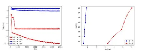
Figure 1: Training loss and loss-width relation of different network for fitting composition functions with different intrinsic dimension. Left: Training loss at each step of network with width W=2 and W=64. Right: the loss-width relation of the network for composition functions with intrinsic dimension t=2 and t=4.

According to the left part,with a larger intrinsic dimensiont,the improvement in the precision by using more units each layer becomes smaller,since the gap between converged loss by networks with different width gets narrower. In another word, a smaller intrinsic dimension may better alleviate the curse of dimensionality, in the sense that the optimal loss decreases faster with an increasing network width. This fact can also be found in the right part of Fig. 1, in which we further depict the relation of log(W) and log(1/∈) obtained for composition function witht=2 and 4.As is shown, the slope int=4 case is bigger thant=2, which again indicates the fact that when learning for a composition function, the gains in converged precision by increasing network width becomes larger if the intrinsic dimension is smaller.Besides, the right part can qualitatively verify the relation (5.1), which can also be written as

Similar results of solving PDEs for composition functions by PINNs have also been plotted in Fig. 2.

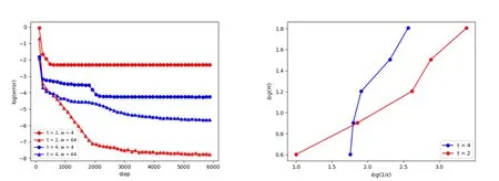
Figure 2: Training loss and loss-width relation of different network for solving (3.1)by PINNs while the true solution is set as composition functions with different intrinsic dimension. Left: Training loss at each step of network with width W=2 and W=64. Right: the loss-width relation of the network for composition functions with intrinsic dimension t=2 and t=4.

6 Conclusions

We have presented an approximation result for composition functions in high dimensions Rd, which reveals that the convergence rate only depends on the intrinsic dimensiontof each composition layer. As an application, we have shown that the error of PINNs method converges to∈with a sampling size ofO(), DNN widthO() and depthO(「log2), which partially solves the curse of dimensionality whent≪d, in the sense that for a fixed-dimension problem, the sampling complexity and the network size will not increase exponentially with decreasing error.

Acknowledgements

This work is supported by the National Key Research and Development Program of China(No.2020YFA0714200),by the Natural Science Foundation of Hubei Province(Nos. 2021AAA010 and 2019CFA007), by the National Nature Science Foundation of China (Nos. 12301558, 12288101, 12125103 and 12071362), and by the Fundamental Research Funds for the Central Universities. The numerical calculations in this paper have been done on the supercomputing system in the Supercomputing Center of Wuhan University.