A New Locking-Free Virtual Element Method for Linear Elasticity Problems

Jianguo Huang, Sen Lin and Yue Yu

1 School of Mathematical Sciences, and MOE-LSC, Shanghai Jiao Tong University, Shanghai 200240, China

2 School of Mathematical Sciences, Institute of Natural Sciences and MOE-LSC, Shanghai Jiao Tong University, Shanghai 200240, China

Abstract. This paper devises a new lowest-order conforming virtual element method (VEM) for planar linear elasticity with the pure displacement/traction boundary condition. The main trick is to view a generic polygon K as a new onewith additional vertices consisting of interior points on edges of K, so that the discrete admissible space is taken as the V1 type virtual element space related to the partition {} instead of {K}. The method is proved to converge with optimal convergence order both in H1 and L2 norms and uniformly with respect to the Lamé constant λ. Numerical tests are presented to illustrate the good performance of the proposed VEM and confirm the theoretical results.

Key words: Virtual element method, linear elasticity, locking-free, numerical tests.

1 Introduction

Robust numerical solution of parameter dependent partial differential equations(PDEs) is a very important topic in scientific computing. A typical example is the linear elasticity problem which involves the Lamé constantsλandμ. Ifλis very large, the material becomes nearly incompressible, which will lead to the so-called volume locking phenomenon when the Courant element is used for discretization(cf. [8]). In the past four decades or more, a huge work has been developed to overcome this difficulty. We refer the reader to [6,7,15,17,19,28,29,32,38,42] and the references therein for details along this line.

On the other hand, the virtual element method (VEM) is a newly proposed numerical method for solving PDEs in recent years, which can be viewed as a generalized finite element method allowing for the use of polytopal meshes (polygons or polyhedra) of very general shape. It was first proposed and analyzed in [2,9,11]and immediately attracted much attention from the research community due to its advantages in handling problems with complex geometries,high-regularity solutions(cf. [21,31]). As far as we know, there have also developed some locking free VEMs for the linear elasticity problem. Letkdenote the order of the virtual element used.The conforming VEMs for this problem were first studied in [10]. However, the conditionk≥2 is required so as to produce locking free optimal error estimates in theH1norm. More recently,a lowest-order locking-free VEM was devised in[37]to remedy this disadvantage by modifying theW1type virtual element technically so that the uniform inf-sup condition holds. This method can be regarded as the extension of the well-known Bernardi-Raugel finite element method (cf. [14]) in general polygonal meshes. In [41], some nonconforming VEMs were proposed for attacking the previous problem in two and three dimensions. It was shown in this paper that ifk≥1 (resp.k≥2), the method is locking-free for the pure displacement (resp.traction) problem. Recently, two kinds of lowest-order locking free VEMs were proposed in [33]. Here, the first one is nonconforming virtual element combined with a special stabilizing term, and the second one is constructed by using the conforming virtual element for one component of the displacement field and the nonconforming virtual element for the other. We mention in passing that there are some other VEMs discussing numerical solution of elasticity problems and other problems in different aspects; see, e.g., [3–5,13,18,23,25–27,34,35,39,40].

In this paper,we are concerned with proposing and analyzing a new lowest-order conforming locking-free VEM for the pure displacement/traction problem,by means of a significant feature of VEMs. The main ideas behind the method include:

1. For a generic polygonal elementKwithNKedges, denoted byits vertices which are numbered in a counter-clockwise order and bythe edge connectingzitozi+1, wherezNK+1:=z1. Then we construct an auxiliary polygon(see Fig. 1), which has the same geometric shape asKbut has more vertices. Precisely speaking, besides the vertices ofK,has additional vertices formed by the internal pointsof edges ofK,which are chosen such that |, whereα∈(0,1) is any fixed constant.It is a significant advantage of VEMs that one can view an interior point of an edge as an additional vertex, so that the difficulty of hanging nodes during adaptivity can be overcome very conveniently (cf. [30]). But here we use the technique to construct locking free VEMs.

2. Based on theV1type virtual element space with respect the partition {}instead of the usual one {K}, a locking free VEM is naturally devised using the ideas in [10] fork≥2.

Under the standard mesh assumption C0 (see Subsection 3.1), we can show the proposed method is locking free and has the optimal convergence order by invoking a new interpolation operator which satisfies the required commutative property and admits the optimal error estimates. We offer several numerical tests to illustrate the performance of the proposed method and confirm its theoretical predictions.

We end this section by introducing some notations for later requirement. We use standard notations for Sobolev spaces and norms (see [1] for more details). LetDbe any open subset of Ω and|D|denote the area ofD. Given a non-negative integerm, we denote the standard Sobolev spaces onDbyHm(D) with norm‖·‖m,Dand semi-norm |·|m,D, and denote theL2-inner product onDby (·,·)D. By convention,H0(D)=L2(D). Let Pm(D) be the set of polynomials of degree less thanmonD. Moreover, we omit the subscript whenD=Ω. For the vector-valued functions or spaces, we use the bold symbols, such asv,L2(Ω),Hm(Ω),Hm0(Ω), etc. Letv=(v1,v2)Tandτ=(τij)2×2be functions of two variables. We define

For any two quantitiesaandb, “a≾b” indicates “a≤Cb” with the hidden generic positive constantCindependent ofλand the mesh size, which may take different values at different occurrences, andabshowsa≾b≾a.

2 The linear elasticity problem

Let Ω⊂R2be a convex polygonal domain with the boundary∂Ω. Given an applied forcef∈L2(Ω), the linear elasticity problem is to find the displacement vectoru=(u1,u2)Tsuch that

whereε=(εij)2×2,εij(u)=(∂iuj+∂jui), and

Here,μandλare the Lamé constants satisfyingμ∈[μ1,μ2] with 0＜μ1＜μ2andλ∈(0,∞), and I is the identity matrix.

The variational formulation of (2.1) is to findu∈V=H10(Ω) such that

where

and

By the well-known Korn inequality (cf. [16]):

it is easy to obtain the boundedness and coercivity ofa(·,·):

which imply that the problem (2.1) has a unique solution by the Lax-Milgram lemma.

Since the first term ofa(·,·) (cf. (2.3)) is related toμ, we write

for later uses.

It is shown in [17]that the following regularity estimate holds for the solutionuof (2.1):

where the hidden constant is independent ofλ.

3 Virtual element methods for the pure displacement problem

In this section, by means of a mesh refinement trick in VEMs, we propose a new lowest order locking-free conforming virtual element method on the fine mesh.

3.1 Mesh assumption and the virtual element space

Let {Th} be a family of decompositions of Ω into polygonal elements. The generic element is denoted byKwith diameterhK=diam(K). For clarity, we work on meshes satisfying the following condition (cf. [9]):

C0.For each elementK, there exists positive constantsγ1andγ2independent ofhKsuch that

·Kis star-shaped with respect to a disc inKwith radius ≥γ1hK;

·the distance between any two vertices ofKis ≥γ2hK.

Due to the large flexibility of the meshes in VEMs,under the above assumption,one easily finds that the mesh can be refined by taking the internal pointmiof each edgeeiof every elementKas a new vertex(see Fig.1). For the new edge,we assumefori=1,2,...,NKfor a given constantα∈(0,1). The resulting fine mesh will be denoted byT*hwith the generic element given by. It’s obvious thatT*hstill satisfies the assumption C0 though the generic constants may change.Here,withbeing the diameter of. It is evident that

Figure 1: The auxiliary polygonsatisfying the mesh assumption C0. The polygonal elements of the fine mesh T *h and the original mesh Th are denoted byand K, respectively. The red circle points denote the original vertices, the blue square points denote the added vertices.

In this paper, we consider the lowest-order conforming virtual element space(VES) defined on the fine meshT*h. To this end, we briefly review the construction method mentioned in [9]. The local scalar virtual element space onis defined as

The local virtual element space for linear elasticity is then given by the tensor product spaceThe corresponding local degrees of freedom (DOFs)are:

·χi∈χ: the values at vertices of

In what follows,denote byVhthe global VES,which is defined elementwise and required that the degrees of freedom are continuous through the interior vertices while zero for the boundary DOFs, i.e.,

3.2 The virtual element method

As in [10], we first introduce the elliptic projectionfor dealing with the first term of (2.3), which is given by

One can check that the functioncan be computed by the given DOFs forv∈V1(). Also,simply write Π1for the related elementwise defined global operator.

Next,let ΠK0be the usualL2orthogonal projection fromL2(K)into the constant space overK. In other words, for allv∈L2(K), ΠK0v=∫Kvdx/|K|. This definition naturally applies to anL2vector valued function. For allv∈H1(K),by integration by parts,

wherenK=(n1,n2)TandtK=(-n2,n1)Tdenote the unit normal and tangent vector to∂Kdetermined by the right hand side quantities, respectively. Hence, for allv∈V1(), we can compute ΠK0divvand ΠK0rotvonly using the function values at the vertices of. Therefore, we treat the second term in (2.3) using the same method in [10] for the casek≥2.

With the help of the above projections, we construct the local computable bilinear form by

where

and

with=2NK.

The locking-free conforming VEM of the variational problem (2.2) is to finduh∈Vhsuch that

where

and the approximation of the right hand side is given by

Remark 3.1.It is worth noting that even on triangular meshes, the proposed lowest-order conforming virtual element does not reduce to the well-known Courant element. In addition, at each edge of a polygonK∈Th, the number of the local DOFs of the virtual element proposed here is one more than that of the virtual element given in [37].

3.3 Stability of the virtual element method

We first recall a classic Korn’s inequality with respect to a star-shaped domain [17,22].

Lemma 3.1.LetD⊂R2beaboundeddomainofdiameterh,whichisstar-shaped withrespecttoadiscofradiusρ.Thenforanyv∈H1(D)satisfying∫Drotvdx=0,thereholds

wherethehiddenconstantConlydependsontheaspectratioh/ρ.

According to the definition of,the above lemma and the Dupont-Scott theory,we can obtain the following stability result.

Lemma 3.2.Forall,thereholdsthestabilityestimate

whichyieldstheerrorestimate

Proof. By settingp=vin the first equation of (3.2) and using the definition of, we easily have

which combined with the triangle inequality gives

By Lemma 3.1, (3.8) and the triangle inequality,

So we derive(3.6). Furthermore,according to the Dupont-Scott theory,there exists a certainq∈(P1())2such that

This, in conjunction with the triangle inequality,q=qand (3.6), leads to (3.7):

This completes the proof.

With the help of Lemma 3.1, we can also derive the norm equivalence and the stability estimate for the proposed virtual element method (3.4), described as follows.

Theorem 3.1.UnderthemeshassumptionC0,forallvh∈Vhtherehold

and

where(vh,vh)isthelocalcounterpartofaμ(vh,vh).

Proof. By the definition ofand Lemma 3.1, one has

According to the norm equivalence in [20],

for anyv∈V1(), and hence

In view of the inverse inequality in [20] and the standard Poincaré-Friedrichs inequality, we further obtain

which together with (3.11) and (3.12) yields the estimate (3.9).

The estimate (3.10) follows readily from (3.9) and the fact that

This completes the proof.

4 Error analysis

For a partitionThand a non-negative integerm, denote by Pm(Th) the set of all broken polynomials related toTh. In other words, for allv∈Pm(Th),v|K∈Pm(K)for allK∈Th. Then, following similar arguments in [10], we can derive an abstract lemma for the error analysis.

Lemma 4.1.Letu∈Vanduh∈Vhbethesolutionsoftheproblems(2.2)and(3.4),respectively.ThenunderthemeshassumptionC0,foranywh∈Vhandfor anypiecewisepolynomialuπ∈(P1(T*h))2,thereholds

whereΠ0divv|K=ΠK0divvforallv∈V, |·|1,histhebrokenH1seminormonΩand

Proof. By settingδh=uh-whand using the triangle inequality,it suffices to bound|δh|1. According to the equivalence (3.10) and Korn’s inequality (2.4), we have the coercivity

The remaining arguments are similar to the ones given in the proof of Theorem 3.2 in [10].

We now prove the locking-free property of the proposed VEM. To this end, we shall introduce a special interpolation operator as presented in the proof of the following lemma.

Lemma 4.2.Forallu∈H10(Ω)∩H2(Ω),thereexistsaVEMfunctionuI∈Vhsuch that

and

Proof. By the definition of ΠK0div and by integration by parts, one has

Then the first relation of (4.3) is equivalent to

Similarly, the second relation of (4.3) is equivalent to

Thus, it suffices to construct a VEM functionuI∈Vhsuch that

We construct the functionuIby determining its DOF values. For any edgeeiofKwith two end pointsziandzi+1withi=1,2,...,NK,there exists one internal pointmisuch that the edgeeiis divided into two subedgesand|ei1|=α|ei|. For the vertices ofK, we define

SinceuIis piecewise linear along∂K, we have

which forces us to define

WriteIKu=uI|Kfor allK∈Th. SinceIKu∈V1(), we have by the inverse inequality and norm equivalence in [20] that

wherep∈meanspis a vertex of.

Under the mesh assumption C0,by connecting the center of the disc used in the star-shaped condition with the vertices ofK, we can obtain a virtual triangulationTKofK,which is quasi-uniform and shape-regular with the mesh sizehK. Moreover,the number of the triangles inTKis uniformly bounded with respect toTh. For all trianglesτ∈TK, it follows from the Sobolev inequality and the scaling argument that

wherehτdenotes the diameter ofτ, which is proportional tohK. This immediately implies

On the other hand,by the Dupont-Scott theory(cf.[16]),for allu∈H2(K)there exists auπ∈(P1(K))2such that

Observing thatIKuπ=uπ, we have by (4.5)–(4.7) that

as required.

which immediately implies

Thanks to Lemmas 4.1-4.2, the projection error estimates (cf. [16]) and the estimate for (4.2) (see (4.8)), we are able to derive the following error estimate which is uniform with the incompressible parameterλ.

Theorem 4.1.LetuanduhbegivenasinLemma4.1.UnderthemeshassumptionC0andtheconditionofregularityestimate(2.5),thereholds

withthehiddenpositiveconstantCindependentofhandλ.

Using the duality argument and following the similar idea for proving Lemma 2.4 in [10], we can establish the optimal error estimate inL2norm. As a matter of fact, introduce an auxiliary problem of (2.1) by findingφ∈Vsuch that

Since the domain Ω is convex, we also have from [17] thatφ∈H2(Ω) which admits the estimate

The variational formulation of (4.10) is to findφ∈Vsuch that

Theorem 4.2.UnderthesameassumptionsofTheorem4.1,thereholds

withahiddenconstantCindependentofhandλ.

Proof. LetφI∈Vhbe the interpolant ofφgiven in Lemma 4.2, andφπ∈(P1(T*h))2the piecewise linear approximation ofφ, respectively. Then it follows from Lemma 4.2, the standard approximation estimate and the regularity result (4.11) that

By (4.12), we obtain

For the second term on the right side of (4.15), we rewrite it as

As usual, letIbe the identity operator. Then, owing to the relation ΠK0divφ=ΠK0divφI, it follows from (4.15) and (4.16) that

Making use of (4.15)–(4.17), we arrive at

Next, we bound the four quantities on the right hand side of (4.18) one by one. It follows from the Cauchy-Schwarz inequality, (4.9) and (4.14) that

By thek-consistency ofaμ,h(·,·), (3.10) and (4.14), we find

Following the similar arguments for deriving (4.8)and using Lemma 3.2 and(4.14),we see that

Applying the Cauchy-Schwarz inequality, Theorem 4.1 (see (4.9)), the regularity results (2.5) and (4.11) gives

The combination of (4.18), (4.19), (4.20), (4.21) and (4.22) leads to the desired estimate.

5 The VEM for the pure traction problem

In this section, we extend our approach to the following pure traction problem:

wherendenotes the unit outward normal to∂Ω. The problem (5.1) is uniquely solvable indefined later if and only iffsatisfies the following compatibility condition (cf. [16,17])

where

We define the admissible space as

which is slightly different from the used space(Ω) defined by (cf. [16])

Here, the first constraint is replaced by an integrand on the boundary∂Ω not the whole domain Ω. The choice here is considered for two reasons, one is to ensure the interpolation of the VEM function lies in the underlying VES, and the other is to make the terms associated with Lagrange multipliers computable in the implementation. One can refer to Subsection 6.1 for details. The continuous variational problem(5.1)is the same as the one given in(2.2),with the function space replaced by. The local VES onis given by, whereis the same as the one given in (3.1), i.e.,

and the global VES given by

The locking-free conforming VEM of problem (5.1) is to finduh∈Vhsuch that

Here, the computable bilinear form and the approximation of the right hand side are the same ones as given in (3.4).

We now establish a similar result as Lemma 4.2.

Lemma 5.1.Forallu∈∩H2(Ω),thereexistsaVEMfunctionuJ∈suchthat

and

Proof. LetuI∈Vhbe the function given in Lemma 4.2. Then it immediately gives

Define

We then have

which indicatesuJ∈.

Since |u-uJ|1=|u-uI|1, the estimate follows from the similar arguments for deriving (4.4).

With the help of the above lemma and following the same arguments in Section 4, we are able to derive the parameter-free error estimates, described as follows.

Theorem 5.1.Letubetheweaksolutionofproblem(5.1)anduhbethediscrete solutionofproblem(5.2),respectively.UnderthesameassumptionsasinTheorem4.2,therehold

and

Here,thehiddenconstantsareindependentofhandλ.

6 Numerical experiments

In this section, we present some numerical tests for the locking-free conforming VEMs (3.4) and (5.2) to confirm the theoretical results.

Letube the exact solution of (2.1) (resp. (5.1)) anduhthe discrete solution of the proposed VEM (3.4) (resp. (5.2)). For the ease of programming, we always chooseα=1/2 in our numerical method. That means, the midpoint of each edge of the polygonal elementKis taken as an additional vertex of. Since the VEM solutionuhis not explicitly known inside the polygonal elements, as in [12], we will evaluate the computable errors by comparing the exact solutionuwith the elliptic projectionuhofuh. In this way,the discreteL2error ErrL2 andH1error ErrH1 are respectively quantified by

6.1 Implementation of the proposed VEM

In this subsection, to help the reader use the numerical method, we present the computer implementation of theL2projection ΠK0div. One can refer to [24] for the numerical realization of other standard terms. LetφT=(φ1,φ2,···,) be the basis functions ofV1() and denote

to be the basis functions of the vector spaceV1(), where

Then the definition ofL2projection ΠK0div can be written in vector form as

where

By integration by parts,

Owing to the Kronecker propertyχi(φj)=δij, the two integrals of the right-hand side can be easily computed by using the trapezoidal rule and the associated local stiffness matrix

will be elementwise assembled.

On the other hand,for the pure traction problem,the discrete admissible function must satisfy the constraints

To impose these constraints,we introduce Lagrange multipliersβi∈R(i=1,2,3)and consider the augmented variational formulation: Find(uh,β1,β2,β3)×R×R×R such that

whereuh=(uh,1,uh,2)T,vh=(vh,1,vh,2)Tand

Letφi,i=1,···,Nbe the nodal basis function of, whereNis the dimension of. Then we can write

Plug the above expression into (6.1), and takevh=φjforj=1,...,N. We have

Let

The linear system can be written in matrix form:

6.2 The pure displacement problem

Test 1.We consider the linear elasticity problem (2.1) on Ω=(0,1)2with homogeneous Dirichlet boundary conditions. The load termfis chosen such that the exact solution of (2.1) is

Case 1.We first consider the convergence with respect to different mesh shapes.To do so, we choose three different sequences of meshes, labeled byM1,M2,M3,as shown in Fig. 2, whereM1is a sequence of meshes composed of unstructured triangles,M2is a sequence of meshes composed of distorted squares, andM3is a sequence of meshes composed of Voronoi polygons. The distorted meshes are obtained by mapping the position(ξ,ζ)of equal squares meshes through the smooth coordinate transformation

And the polygonal meshes are generated by the MATLAB toolbox–PolyMesher introduced in [36].

Letμ=1 andλ=106. We display the nodal values of the elliptic projection Π1uhonM3in Fig. 3, from which we observe that the numerical solutions are well matched with the exact ones. TheH1andL2errors computed as functions of the mesh sizehfor the mesh sequencesare depicted in Fig.4 as a log-log plot.For each fixed pair (λ,μ), the convergence rate with respect tohis estimated by assuming Err(h)=chαand computing a least squares to fit this log-linear relation.We see that the errors ErrH1 and ErrL2 converge at the optimal rateO(h1) andO(h2) respectively, and are not affected by the shape of the mesh discretization. It is worth noting that, the proposed VEM shows a satisfactory stability with respect to the nearly incompressible case (λ=106).

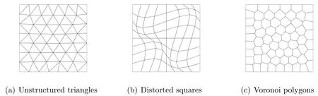
Figure 2: Three families of meshes in Test 1.

Figure 3: Numerical and exact solutions for λ=106 on one polygonal mesh of M3 in Test 1 (left:Mesh512, middle: numerical solution, right: exact solution).

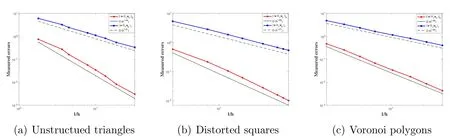
Figure 4: L2 and H1 errors for λ=106 on three different sequences of meshes in Test 1.

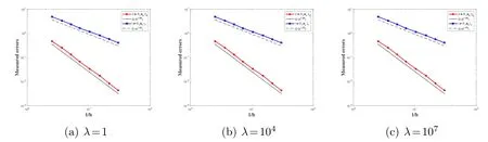
Figure 5: L2 and H1 errors for λ∈{1,104,107} on polygonal meshes M3 in Test 1.

Case 2.We next investigate the locking-free property of the proposed VEM,i.e.,the robustness with respect to the choice ofλ. In this case,we only focus on considering the Voronoi polygonal meshesM3.

Letμ=1 andλ∈{1,104,107}. The convergence graphs of the errors ErrH1 and ErrL2 for different values ofλare displayed in Fig. 5, and the corresponding errors ErrH1 and ErrL2 are shown in Table 1. We observe that all the errors are almost the same and the method converges with the optimal rates, which is in well agreement with the theoretical predictions in Theorems 4.1 and 4.2.

Table 1: H1 and L2 errors for λ∈{1,104,107} on polygonal meshes M3 in Test 1.

Furthermore, we takeλ∈{10j,j=0,1,···,7} on a fixed mesh inM3withh=0.065690. As shown in Table 2, the errors ErrH1 and ErrL2 are insensitive to the choice ofλ, thus the proposed VEM is robust with respect toλ, i.e., it is volumelocking-free.

Table 2: H1 and L2 errors for different values of λ on one fixed mesh of M3 in Test 1.

Table 3: Convergence rate w.r.t. H1 norm for λ∈{1,104,107,1010} on meshes M3 in Test 2.

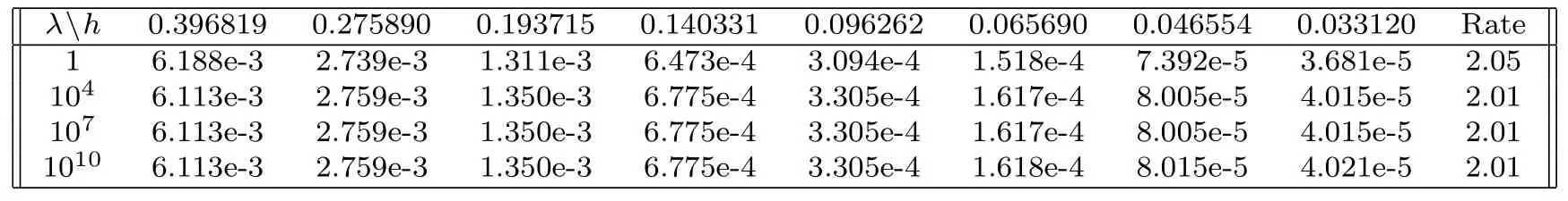
Table 4: Convergence rate w.r.t. L2 norm for λ∈{1,104,107,1010} on meshes M3 in Test 2.

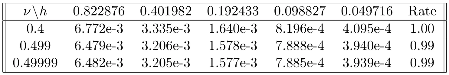
Table 5: Convergence rate w.r.t. H1 norm for ν ∈{0.4,0.499,0.49999} on meshes M4 in Test 4.

Table 6: Convergence rate w.r.t. L2 norm for ν ∈{0.4,0.499,0.49999} on meshes M4 in Test 4.

6.3 The mixed boundary conditions

Test 2.We solve the following linear elasticity problem on Ω=(0,1)2with general boundary conditions:

where, Γ2=｛(x1,x2)|0 ≤x1≤1,x2=0and Γ1=∂ΩΓ2. We select the load termfand the boundary conditions such that the analytical solution of problem (6.2)(cf. [38]) is

Here, the first term is divergence-free, but the second term provides a constant divergence (2/λ). It is clear that divu=0 asλtends to infinity.

We takeμ=0.5 andλ∈{1,104,107,1010} on Voronoi polygonal meshesM3. The nodal values of the elliptic projection Π1uhforλ=1010are shown in Fig. 6. The results and convergence graphs of the two errors ErrH1 and ErrL2 versus the mesh sizehfor different choice ofλare illustrated in Tables 3-4 and Fig. 7, respectively.As observed, the optimal rates of convergence are achieved for both cases.

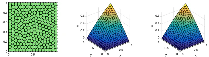
Figure 6: Numerical and exact solutions for λ=1010 on one polygonal mesh of M3 in Test 2. (left:Mesh512, middle: numerical solution, right: exact solution).

Figure 7: L2 and H1 errors for λ∈{1,104,107,1010} on polygonal meshes M3 in Test 2.

6.4 The completely incompressible limiting problem

Test 3.We now consider the completely incompressible problem which exact solution is given by

It’s easy to check that divu=0 andfis independent ofλ. Now we investigate the impact of Lamé constantλon two different sequences of meshes composed by Voronoi and distortion polygons, respectively. Letμ=1 andλ=1010.

The numerical solutions are well matched with the exact ones even on distortion polygonal meshes as observed in Fig. 8. From the convergence graphs of the errors ErrH1 and ErrL2 forλ=1010on two families of polygonal meshes displayed in Fig.9,we still obtain a satisfactory result that the optimal rates of convergence are achieved for both subdivisions in the completely incompressible limiting case.

Figure 8: Numerical and exact solutions for λ=1010 on one distortion polygonal mesh in Test 3. (left:Mesh512, middle: numerical solution, right: exact solution).

Figure 9: L2 and H1 errors for λ=1010 on Voronoi and distortion polygonal meshes in Test 3.

6.5 A cantilever beam

Test 4.Next, we are concerned with a linear elasticity problem (6.2) on a rectangular beam that has lengtha, heightband unit thickness. As shown in Fig. 10, the beam is subject to a couple at one end and a linearly varying load with magnitudeFat the free end.

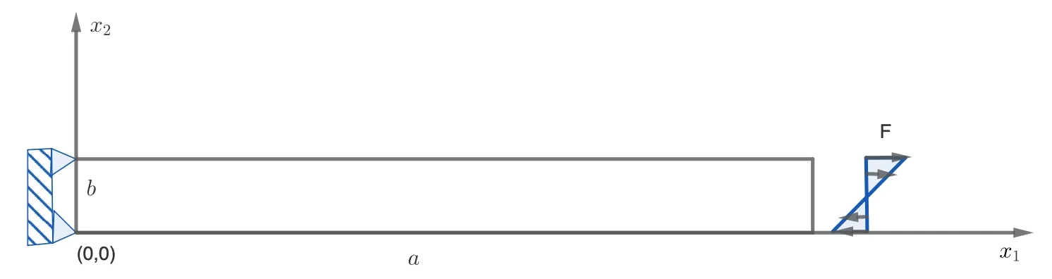
Figure 10: A rectangular beam with length a and height b is coupled at the left end and subject to a linearly load at the right end in Test 4.

Along the edgex=0,the horizontal displacement is zero. At the lower-left corner(i.e,the point(0,0))and the upper-left corner,the vertical displacement is also zero.In other words,

We ignore the beam’s own weight, so there is no body force exerting on the beam, i.e.,f=0. Note that the Lamé constantsμandλare given by

whereEis the elasticity modulus andνis Poisson’s ratio. Asνtends to 1/2,λtends to infinity. It is known from [29] that the exact solution for displacementuis

where

It is clear that

so the upper half of the beam(y＞b/2)is stretched, whereas the lower half(y＜b/2)is compressed. Moreover,∇·u→0 asν→. It follows from direct calculations that

Hence the maximum of the normal stress in thex-direction is max(σ11)=F.

An interesting phenomenon in this test is that many quantities, e.g., displacementuand stressσ, are actually independent of the beam lengtha.

In our numerical tests, we seta=10,b=1,E=1000,F=5 but varyνamong 0.4, 0.499 and 0.49999 (resp.λamong 1.42857e+3, 1.66444e+5 and 1.66664e+7).We use a sequence of Voronoi polygonal meshesM4with (10n)×nelements, wheren=2,4,8,16,32, respectively. The profiles of the elliptic projection Π1uhonM4forν=0.49999 on an 80×8 Voronoi polygonal mesh is displayed in Fig. 11. In this case, one can clearly observe the symmetry of the numerical displacement across the middle liney=1/2 and the downward bending in the beam, due to the linearly varying load on the free end.

Figure 11: Numerical solution for ν=0.49999 on a 80×8 Voronoi polygonal mesh in Test 4.

Figure 12: L2 and H1 errors for ν ∈{0.4,0.499,0.49999} on polygonal meshes M4 in Test 4.

The results and convergence graphs of the two errors ErrH1 and ErrL2 versus the mesh sizehfor different choice ofνare illustrated in Tables 5-6 and Fig. 12, respectively. As observed,the convergence rates for ErrH1 and ErrL2 are respectively 1st and 2nd order, as expected, regardless of the value of Poisson’s ratioν. In this case, one can clearly observe the symmetry of the numerical displacement across the middle liney=1/2 and the downward bending in the beam, due to the linearly varying load on the right (free) end. Totally speaking, we get very good numerical approximations with our proposed locking-free method in this example.

6.6 Cook’s membrane

Test 5.Finally, we consider Cook’s membrane problem, which is often used to test the performance of numerical methods for nearly incompressible solid materials under combined bending and shear. For this benchmark example, the geometric domain is a convex quadrilateral with four vertices(0,0),(48,44),(48,60)and(0,44)as shown in Fig.13(a). The panel is clamped on the left side(x=0)and subjected to a shearing loadσn=gN=(0,g)T,whereg=6.25 is the vertical traction force per unit length. The remaining two sides are traction-free with vanishing volume forcef.Besides,the Lamé constants are given byμ=E/(2(1+ν))andλ=Eν/((1+ν)(1-2ν)),where we set the elasticity modulus and Poisson’s ratio asE=250 andν=0.4999,respectively.

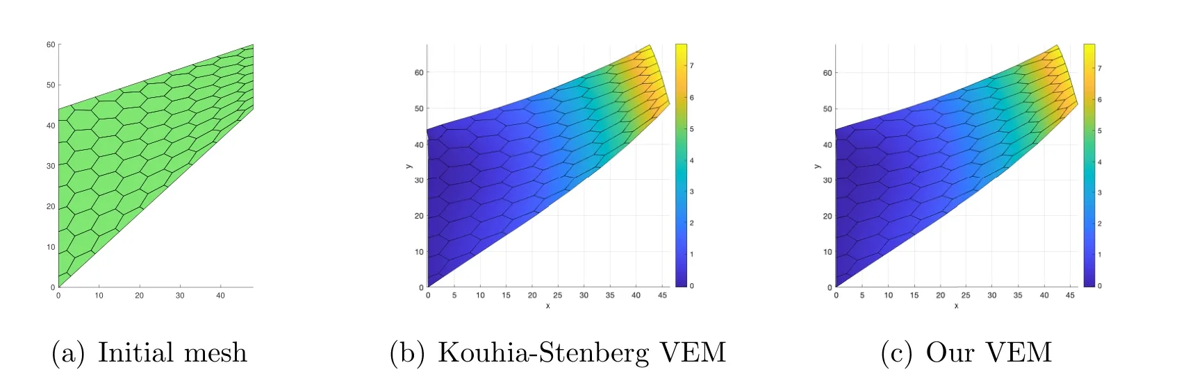
Figure 13: Initial and deformed meshes of the Cook’s membrane problem on the polygonal mesh in Test 5.

Thus, Cook’s membrane problem is to find the displacement fieldusuch that

We now solve the problem (6.3) by our locking-free VEM and the Kouhia-Stenberg VEM in [33], respectively. To show the flexibility of mesh selection,we choose two different initial meshes, one is composed of Voronoi polygons, and the other is a typical non-convex tessellation referred as the Guelve mesh (see Fig. 14(a)). The initial mesh and the deformed panel solved by the two VEMs for the above two meshes are shown in Fig. 13 and Fig. 14, respectively. Here, the plot is deformed due to the elliptic projectionuh, that is, the coordinates (x1,x2)Tof the vertices are changed to(x1+u1,h,x2+u2,h)T,and the colorbar corresponds to the values ofu2,h. We can observe that the performance of our method is consistent with the one from the Kouhia-Stenberg VEM.Moreover, even if the element of the initial mesh is non-convex,we can also get a desired numerical solution in the nearly incompressible case.

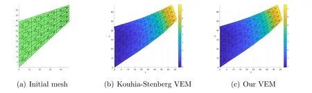
Figure 14: Initial and deformed meshes of the Cook’s membrane problem on the Guelve mesh in Test 5.

7 Conclusions

We propose a new locking-free conforming VEM in the lowest order case for solving linear elasticity problems. The key is to view the meshKaswhich is formed by including an interior point of each edge as an additional vertex. Then the method in [10] can be extended to the case ofk=1, ifV1(K) is replaced byV1(). Another approach to developing a similar method is to use the static condensation for theV2method given in [10]. Compared to this method, our approach is simple in construction and easy in programming.

Acknowledgements

The authors would like to thank the referees for valuable comments which greatly improved an early version of the paper. The work of JH was partially supported by NSFC (Grant No. 12071289) and the Fundamental Research Funds for the Central Universities.