A Linearized Adaptive Dynamic Diffusion Finite Element Method for Convection-Diffusion-Reaction Equations

Shaohong Du, Qianqian Hou and Xiaoping Xie

1 School of Mathematics and Statistics, Chongqing Jiaotong University,Chongqing 400074, China

2 School of Mathematics, Sichuan University, Chengdu, Sichuan 610064,China

Abstract. In this paper, we consider a modified nonlinear dynamic diffusion(DD) method for convection-diffusion-reaction equations. This method is free of stabilization parameters and capable of precluding spurious oscillations. We develop a reliable and efficient residual-type a posteriori error estimator, which is robust with respect to the diffusivity parameter. Furthermore, we propose a linearized adaptive DD algorithm based on the a posteriori estimator. Finally,we perform numerical experiments to verify the theoretical analysis and the performance of the adaptive algorithm.

Key words: Convection-diffusion-reaction equation,dynamical diffusion method,residualtype a posteriori error estimator, adaptive algorithm.

1 Introduction

Let Ω⊂Rd(d=2,3) be a polygonal/polyhedral domain with boundary Γ=∪,where ΓD∩ΓN=Øandmeas(ΓD)＞0. We consider the convection-diffusion-reaction problem

whereurepresents the quantity being transported,0＜ε≪1 the(constant)diffusivity,β∈[W1,∞(Ω)]dthe velocity field, 0≤σ∈L∞(Ω) the reaction coefficient,f∈L2(Ω)the source term, n the outward unit normal vector along Γ, andg∈L2(ΓN) the Neumann boundary condition.

We first make the following two assumptions:

(D1) There are two nonnegative constantsγandcσ, independent ofε, satisfying

this assumption ensures that we can simultaneously handle the cases ofσ≠0 andσ=0 (cf. [53]), with the latter case corresponding toγ=0 andcσ=0.

(D2) The Dirichlet boundary ΓDincludes the inflow boundary, i.e., ΓD⊃{x∈Γ:β(x)·n＜0}.

It is well-known that classical finite element methods usually give rise to numerical oscillations for convection-dominated convection-diffusion equations, due to local singularities arising from interior or boundary layers (cf. [12–14,23,44,45]). In order to overcome the limitations of the Galerkin mehtods, a lot of stabilized finite element methods have been developed,such as Streamline-Upwind/Petrov-Galerkin(SUPG) methods [9], Galerkin-Least-Squares methods [32], Residual-Free Bubbles methods[5],Variational Multiscale(VMS)methods[7,8,23,26–29,33,34,36,41],and Discontinuous Galerkin type methods [2,10,15,18,19,24,35]. By suitable designing stabilization parameters, these linear stabilized methods are capable of producing accurate and oscillation-free numerical solutions in regions where the exact solution has no abrupt changes. However, they do not preclude spurious oscillations in the neighbourhood of sharp layers.

To get rid of the local oscillations,many nonlinear stabilized finite element methods have been developed by adding an extra diffusivity term to the formulation to recover the monotonicity of the continuous problem[1,11,20,25,31,37,48–51]. Such methods lead to nonlinear systems due to the introduction of nonlinear artificial dissipation dynamically adjusted in terms of the notion of scale separation. Among the nonlinear stabilized methods, the Dynamic Diffusion (DD) method [50,51] is a parameter-free one which is based on the VMS framework and consists of adding locally and dynamically a nonlinear artificial diffusion so as to guarantee stability of the resolved scale solution.

In order to resolve the layers, it is appealing to use adaptive meshes based on a special robust a posteriori estimator (the ratio of constants in the upper and lower bounds are independent ofε), since the layers are resolved only when the mesh size arrives at the width of layers. However, it is a challenging task to design a robust a posteriori estimator for this type problem, as the constants occurring in the estimators usually depend on the small diffusion parameterε. It is known that a proper norm is crucial to obtain robust a posteriori estimator. In what follows we simply look back at the process of finding such a norm. Verfürth [52]firstly considered anε-weighted energy norm and showed that the estimator was robust when the local Péclet number was not very large, and later further studied robust estimators where the numerical error is evaluated in anadhocnorm [53].Sangalli [47] applied an interpolated norm (an norm on the interpolated space of function spaces)to develop a residual-type a posteriori estimator for one-dimensional case, and proved that the estimator was robust up to a logarithmic factor with respect to the global Péclet number. Du and Zhang [21] introduced a dual norm and proved that Sangalli’s estimator was uniformly robust with respect toεandγ.In [38] John and Novo discussed the natural SUPG norm and analyzed a robust a posteriori error estimator under some hypotheses. We also refer to [4,40,43,46] for several works on the generalization of the approach presented in [52].

To the authors’ knowledge, so far there is no a posteriori error estimate (in special robust estimator) for the DD method in the literature. There are two main difficulties in the a posteriori error analysis: One is how to find a suitable norm to measure the numerical error caused by the artificial dissipation; the other is what controls the nonlinear artificial dissipation term. Inspired by the dual norm introduced in [21], we introduce a weak norm (dual norm) and use it to construct the control component of the artificial dissipation term. We then develop a residual-type error estimator, which is proved to be reliable, efficient, and robust with respect to the diffusion parameterε. As the DD method leads to a nonlinear system in each iteration step, we present a linearized adaptive algorithm, where the artificial dissipation term is calculated by using the numerical solution of the previous iteration step.

The rest of this paper is organized as follows. Section 2 gives notations and weak formulations of the model problem. Section 3 presents the modified DD method.Section 4 is devoted to the construction of residual-type a posteriori estimator and the analysis of its reliability and efficiency. Finally, Section 5 provides some numerical tests.

2 Notation and weak formulation

For any bounded domainωand nonnegative integerm, we introduce the usual Sobolev spaceHm(ω) onωwith norm ||·||m,ωand semi-norm |·|m,ω. In particular,H0(ω)=L2(ω) is the space of square integrable functions. We use (·,·)m,ωto denote the inner product ofHm(ω)with(·,·)ω=(·,·)0,ω. Whenω=Ω,we set||·||m:=||·||m,Ω,|·|m:=|·|m,Ωand (·,·):=(·,·)Ω. We also set

For any integerk≥0, we denote byPk(ω) the set of all polynomials onωwith degree no greater thank. LetThbe a shape regular triangulation of Ω into triangles/tetrahedrons. Denote byhthe mesh-size function withh|T=hT:=diam(T) for anyT∈Th.

Let

be the usual linear element space, andψTbe the bubble function of degreed+1 defined in each elementT. Introduce finite dimensional spaces

Notice that in a two-scale methodVbis the unresolved(fine)scale space whereasVDhis the resolved (coarse) scale space, andVbis defined by using the bubble functions to reduce the computational cost.

LetEΩbe the set of interior edges/faces of elements inTh,andEDandENbe the sets of boundary edges/faces on ΓDand ΓN, respectively. ThenEh:=EΩ∪ED∪ENis the set of all edges/faces of elements inTh. Denote byETthe set of edges (faces ifd=3) ofT, bythe union of all elements inThsharing at least one point withT,and byωEthe patch of an edge (face)E∈Eh(i.e., the union of all elements inThsharing the edge (face)E).

We define the jump of a functionv∈H1(Th)(“broken” Sobolev space)as follows:

Let nEbe the outward unit normal vector to the edge/faceEofT+ifE=T+∩T-,in special, nEthe outward unit normal vector to the edge/faceEofTifE∈ET∩(ED∪EN).

Throughout this paper, we usecandci,i=1,2,..., to stand for generic positive constants, independent of the (constant) diffusivityεand mesh sizeh, which may take different values at different places. We also use the notationA≾Fto representA≤cF.

We introduce a bilinear formB(·,·) onH1D(Ω)×H1D(Ω) by

Then the standard variational formulation of (1.1) reads: findu∈H1D(Ω) such that

Define a norm‖·‖EonH1Dby

Then the use of the Dirichlet boundary condition, data assumptions (1.2) and integration by parts implies the coercivity and boundedness ofB(·,·), i.e.,

and

for∀v,w∈H1D(Ω), which ensure that (2.1) admits a unique solutionu∈H1D(Ω).

3 A modified DD method

We decompose the velocity fieldβinto the resolved (coarse) scaleβhand the unresolved (fine) scaleβb, i.e.,β=βh+βb, and introduce the kinetic energy related to the unresolved scale by

The idea of the original DD method [51] is to minimize the kinetic energy under the constraint of the vanishing residual, i.e., solve the following local optimization problem:

whereuhis the resolved scale solution. This optimization problem gives a subgrid velocity fieldβbat each elementTwith [48,51]

where

is the residual of the resolved scale solution. For eachT∈Th, denotePeTthe Péclet number by

Then the amount of the additional diffusivity required to dissipate the kinetic energyEkis given by [51]

Introduce a linear projection operatorsuch that

The artificial diffusionξT(uh)(on each element)then defines a local nonlinear operatorDT(κh(·);·,·) by

The original DD method reads: Find

such that

Notice that the local operatorDT(κh(uhb);uhb,vhb)depends nonlinearly on the residual of the resolved scale solutionuh, where the artificial diffusionξT(uh) is large in the zones where the solution is not sufficiently resolved, but almost vanishing in smooth regions or when the diffusion behavior is dominant. Henceforth, the local operatorDT(·;·,·) can switch freely between these two situations, which makes the original DD method be consistent and parameter-free. As the subgrid scale spaceVbis defined by using bubble functions,its degrees of freedom can be locally eliminated(cf. [51]).

Since the local nonlinear operatorDT(·;·,·) defined by the artificial diffusionξT(·)does not have an upper bound, the existence of approximate solutions can not be guaranteed. In order to circumvent this difficulty, Santos et al. [50] gave two alternative variants of the artificial diffusionξT(·):

whereτis an appropriate constant, e.g.,τ=‖f‖0,T. This modification of the artificial diffusion allows for the upper and lower bounds of the corresponding local nonlinear operatorDT(·;·,·), hence the existence, stability, and convergence of discrete solutions follow by using similar approaches in the analysis of nonlinear finite element methods; see [3,11,39,42,49].

We note that the choice of the artificial diffusion (ξT(uh) on each element) is determined by the artificial dissipation termβb, andβbis obtained by minimizing the kinetic energyEk. The local optimization problem (3.1) is reduced to an unconstrained minimization problem when‖∇uh‖0,T=0. Obviously,the problem(3.1)has a unique solutionβb=0 in this case, and this makes the amount of the additional diffusivityξT(uh) vanish. However, the choice (3.4) or (3.5) of the artificial diffusivityξT(uh) excluded such a situation. To remedy this, we modify (3.4) and(3.5) respectively as

4 A posteriori error estimates

4.1 Some preliminary results

Notice that theε-weighted energy norm‖u‖Etends to theL2normγ1/2‖u‖0asεtends to zero. To describe the first-order derivatives in the reduced form ofε=0,a relatedH1/2-norm was incorporated into theε-weighted energy norm in [21] to define a norm |||·||| with

Since this norm is equivalent to theH1-norm, the bilinear formB(·,·) leads to a dual norm

We mention that the norm |||·|||*can be replaced by the computable norm |||·|||when convection dominates, since they are equivalent (cf. [22]).

LetIDh:L2(Ω)→VDhbe the Clemént interpolation operator, and there holds the following locally stable estimate (cf. [16,17,47,52])

We recall the approximation properties ofIDhin the sense of norm |||·||| (cf. [21,Lemma 3.1]):

Lemma 4.1.Foranyv∈H1D(Ω),lethbethemesh-sizefunctionand|||v|||bedefined by(4.1).Thenthereholdthefollowingestimates:

The success of DD method is due to the introduction of the local nonlinear operator. In order to see its contribution to a posteriori indicator clearly, we need to estimate it alone.

Lemma 4.2.Forv∈H1D(Ω),letIDhvbeitsCleméntinterpolationofvinVDh.Thenforanyuhb=uh+ub,thereholds

Proof. By the definition(3.2)ofDT(·;·,·),the propertyκh(uhb)=uhand the Cauchy-Schwarz inequality we have

This estimate, together with the choice (3.6) or (3.7) of artificial diffusion and the local stable estimate (4.3) withl=m=1, yields

In light of (4.6), the inverse estimate and the local stability estimate (4.3) withl=m=0 we also have

Moreover, from (4.6) and the local shape regularity it follows

Combing (4.7), (4.8) and (4.9) yields the desired estimate (4.5).

Finally, we cite a lemma from [21, Lemma 3.2].

Lemma 4.3.ForallT∈ThandE∈εh,letψTandψEbetwobubblefunctions(cf.[53]fordetails)withrespecttoTandE,respectively,anddefinetheresidual weightsαTandαEby

Thenforallv∈Pk(T)andσ∈Pk(E),wehave

4.2 A posteriori error estimate: reliable upper bound

In this subsection, we shall define our a posteriori error estimator and prove its reliability in the norm (4.2). For anyT∈Th, we begin with the standard elementwise residual

and edge/face residual

where,uhbis the solution of the DD method (3.3) and Δuhbis interpreted as the Laplacian applied touhb|T. Then we introduce the element-wise indicator

Theorem 4.1.Letuanduhbbethesolutionsof(2.1)and(3.3)withtheartificialdiffusion(3.6)or(3.7),respectively.Thenthereexistsapositiveconstantc6independentofh,εandγ,suchthat

Proof. Applying integration by parts on each elementT∈Thfor anyv∈H1D(Ω),from(2.1) we have

Subtracting (3.3) from (2.1) withvhb=IDhv, we obtain

Combining (4.13) and (4.14) yields

Notice that

We have from (4.4a) and (4.4b) that

and

By (4.5) we get

Using the definition(4.2)of|||·|||*and(4.15)-(4.18), we obtain the desired estimate(4.12).

Remark 4.1.The componentsαT‖RT‖0,TandαE‖RE‖0,Ein the element indicatorηTreflect the approximation degree ofVDhbtoH1D(Ω), and the componentαT‖R(uh)‖0,Tis the contribution of artificial dissipation to the a posterior indicator,which justifies the DD method.

Remark 4.2.On one hand, although the dual norm |||·|||*can not be calculated directly,it may be approximately replaced by|||·|||when convection dominates. On the other hand,the a posterior estimator reflects the degree of approximation to the error.

4.3 Analysis of efficiency

In this subsection, we shall analyze the efficiency of the a posteriori error estimator by following a similar idea as in the proof of [21, Theorem 5.1].

Let Πkbe theL2-projection operator onto piecewise polynomial space of degree at mostk(k≥2), and set

Define an oscillation of data by

where

Lemma 4.4.Denote

Thenthereexistsapositiveconstantc7dependingontheshaperegularityofthe mesh,suchthat

Proof. Define a wave functionwhby

where the constantsγ1andγ2will be determined later. From (4.10a), (4.10b) and(4.10e), we have

where in the last inequality, we have used the estimate

Notice that the following facts will be used frequently in our proof:

·The support ofψTintersects the support of at most 2ddifferentψE’s;

·The support ofψEintersects the support of at most twoψT’s;

·The support ofψEintersects the support of at most 2d-2 otherψE’s.

From the Young’s inequality we have

which, together with (4.22), gives

Now we choose

which satisfy

By the triangle inequality and property ofL2-projection we get

Combining (4.23) and (4.24) yields

Notice that

Applying the property ofL2-projection, (4.10e), and the Hölder’s inequality, we obtain

where in the last inequality we have used the estimate

Collecting (4.25)-(4.27) and using the definition (4.2) of the dual norm |||·|||*, we get

where the constantc8=1+2dmax{1,c5}max{γ1,γ2}.

In what follows, we analyze the norm |||wh||| defined by (4.1). SinceαTis element-wise constant andαEis a constant on each patchωE, forwh∈H1D(Ω), we have

Moreover, we have the estimate

By the definition ofε-weighted energy norm ||·||E, (4.10c), and the property ofL2-projection, we obtain

From (4.10c) and (4.10d) we get

Similarly, we have

Collecting (4.29)-(4.33) yields

From the inverse estimate it follows

Due toα2K≤hK, we have

From the shape regularity and the factαE≤1 we get

and

Combining (4.35)-(4.39) yields

which, together with (4.34), leads to

where

Finally, letc7=2max(c8,c10), and the desired estimate (4.20) follows from (4.28)and (4.40) directly.

Lemma 4.5.Denote

Thenthereexistsapositiveconstantc11dependingontheshaperegularityofthe mesh,suchthat

Proof. Sinceη2does not contain the edge/face residual, we can define a wave function, similar to (4.21), which only has the element residual. By following the same routine as in the proof of Lemma 4.4,we can obtain the desired estimate(4.41).

Theorem 4.2.Letuanduhbbethesolutionsof(2.1)and(3.3)withtheartificial diffusion(3.6)or(3.7),respectively,letηTbeanelement-wiseindicatordefined in(4.11),andletoschbeanoscillationofdatadefinedin(4.19).Thentheerror betweenuanduhcanbeboundedfrombelowbytheestimatorinthefollowingsense:

wheretheconstantc12dependsonlyonc7andc11.

Proof. By (4.20) and (4.41) we have

which gives the desired estimate (4.42).

Remark 4.3.Since the DD method is actually a two grid method,both the resolved scale solutionuhand the unresolved scale solutionubmake contributions to the a posteriori estimator, just as the efficiency estimate (4.42) demonstrates.

5 A linearized adaptive algorithm

Since the DD method is actually a nonlinear finite element method, one needs to solve a nonlinear system in each iteration step of an adaptive algorithm and the cost of computation is expensive. To avoid solving a nonlinear system, in this section we develop a linearized adaptive DD (LADD) algorithm, in which the artificial dissipation term is calculated using the numerical solution at the previous iteration step.

To describe the LADD algorithm, we replace the subscripthby an iteration counterk≥0, e.g.,

etc.. LetT0be a shape regular triangulation, the basic loop of LADD is then given by the following iterations:

Firstly, use the SUPG method to get a solutionu0overT0as an initial value,namely,u0,b=u0. Then setk=0 and iterate:

(1) Calculate the additional diffusivity quantityξT(uk) on eachT∈Tk.

(2) Solve the following linear system: finduk+1,b, such that

for anyvk,b=vk+vb.

(3) Compute the a posterior indicatorηTon each elementT∈Tk.

(4) Apply the Dörfler marking to select the elements to mark.

(5) Generate a conforming triangulationTk+1,according to certain refinement rule such as the longest edge bisection.

(6) Setk=k+1.

Remark 5.1.Note that LADD is actually a standard algorithm that employs only the indicators {ηT}T∈Tk, but it neither marks the oscillation nor needs the interior node property.

Remark 5.2.In the LADD algorithm the SUPG method is applied to get an initial solutionu0. In fact, it still works to use other methods to get initial data.

6 Numerical experiments

In this section, we use two numerical examples to verify the performance of the LADD algorithm.

6.1 An example with boundary layer

We take Ω=(0,1)×(0,1)and chooseβ=(1,1)andσ=1. This choice ofβandσgivesγ=1. We setu=0 on Γ and select the right-hand sidefso that the exact solution of (1.1) is given by

Although the exact solutionu(x,y) is smooth, it has boundary layers of widthO(ε)atx=1 andy=1. This example is suitable to test whether the estimator is able to capture steep gradients in the boundary layer regions.

Our initial mesh consists of eight isosceles right triangles. In the LADD algorithm, we employ the “longest edge” refinement to obtain an admissible mesh.

Figs. 1 and 2 show the mesh refinements of several iteration steps in case ofε=10-6and the marking parameterθ=0.5. We can see that the refinement concentrates around the boundary layers atx=1 andy=1. Thus the predicted estimator captures well the boundary layers of the solution. The second picture of Fig. 2 reports the approximation solution touover an adaptively refined mesh with 32594 triangles.

Figure 1: The mesh (left) after 6 iterations with 284 triangles and the mesh (right) after 8 iterations with 849 triangles: ε=10-6 and the marking parameter θ=0.5.

Figure 2: The mesh (left) after 9 iterations with 1381 triangles and the approximation solution (right)to u over the mesh after 16 iterations with 32594 elements: ε=10-6 and the marking parameter θ=0.5.

Figure 3: The estimated and actual errors versus the number of elements over uniformly and adaptively refined meshes in case of ε=0.1 (left), and the actual error versus the number of elements over adaptively refined meshes in case of ε=10-6 (right): the marking parameter θ=0.5.

We can observe that the numerical solution has almost no oscillations around the boundary layers. This shows that on one hand, the DD method almost precludes spurious oscillations over adaptive meshes,and on the other hand,it does not require the adjustment of stabilization parameter in terms of differentε,βandσ.

Fig. 3 reports the estimated and actual errors of numerical solutions versus the number of elements over uniformly and adaptively refined meshes, a solid line of log-log slope 0.5 is included in each plot to demonstrate the convergence rate of numerical errors. Here, the errors are measured in the energy norm calculated by a 7-point Gauss rule in each triangle. The first picture of Fig. 3 shows that the estimated and actual errors arrive at their optimal convergence rate over uniformly and adaptively refined meshes forε=0.1, since the width of the boundary layers is not small. The second picture of Fig. 3 shows that numerical errors over adaptively refined meshes decrease more rapidly than those over uniformly refined meshes,since the boundary layers over adaptively refined meshes are resolved better than over uniformly refined meshes for very small diffusivityε=10-6. Simultaneously,this shows that one can substantially reduce the number of unknowns necessary to obtain the prescribed accuracy by using the proposed a posteriori error estimator and the adaptively refined meshes.

6.2 The Hemker problem

In this example,we consider the Hemker problem[30]with minor modification. This advection-diffusion problem is defined in a domain comprised of the exterior of the unit rhombus. We set

β=(1,0),f=0,ε=10-4, andσ=0. The Dirichlet boundary conditions are given by

On the rest of the boundary, we set homogeneous Neumann conditions. This scenario gives rise to an interior layer around the unit rhombus that is predominantly advected downstream from the rhombus,forming a practically constant wake. However, the true solution for the Hemker problem is unknown.

We start with an initial mesh consisting of 140 right triangles, and utilize the “longest edge” refinement to obtain an admissible mesh, and carry out the LADD algorithm.

Figs. 4 and 5 report the adaptive meshes generated by 3 and 4 iterations, respectively, in case of the marking parameterθ=0.8. We can see that the refinement concentrates around the unit rhombus boundary and the linesy=±1, and that the spurious oscillations around the interior layers are almost excluded. These indicate that the predicted error estimator captures well the interior layers. We point out that no stabilization parameter is required to properly choose in the LADD algorithm.

Fig. 6 reports the estimated errors versus the number of elements in adaptively refined meshes forε=10-1, 10-2(left) and forε=10-3, 10-4(right) with the marking parameterθ=0.5. We can observe that the a posteriori estimator has similar performance for different perturbed parameterε, and that the estimated error depends on the degree of freedom uniformly inε.

Figure 4: The mesh (left) after 3 iterations with 2084 triangles and the corresponding approximation solution (right) to u: ε=10-4 and the marking parameter θ=0.8.

Figure 5: The mesh (left) after 4 iterations with 5306 triangles and the corresponding approximation solution (right) to u: ε=10-4 and the marking parameter θ=0.8.

Acknowledgements

This work was supported in part by the Education Science Foundation of Chongqing (KJZD-K201900701), project supported by Scientific and Technological Research Program of Chongqing Municipal Education Commission (Grant No. KJZD-M202300705), and the National Natural Science Foundation of China(No. 12171340).

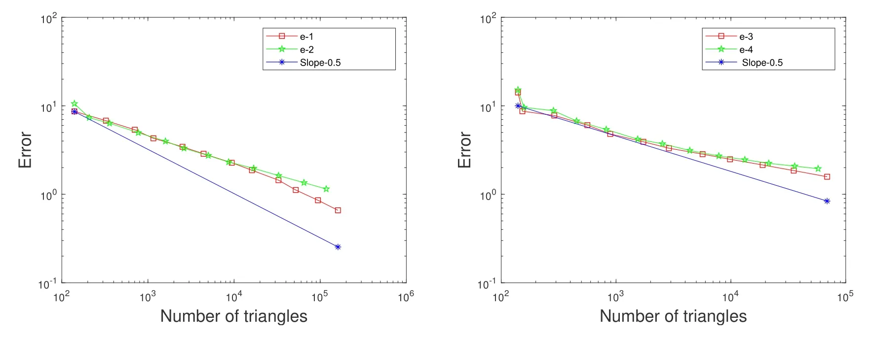
Figure 6: The estimated errors versus the number of elements over adaptively refined meshes: ε=10-1, 10-2 (left)and ε=10-3, 10-4 (right),the marking parameter θ=0.5. Here’10-m’is abbreviated as ’e-m’ for m=1,2,···,4.