An Iterative Thresholding Method for the Heat Transfer Problem

Luyu Cen and Xiaoping Wang,2,3,*

1Department of Mathematics, Hong Kong University of Science and Technology, Clear Water Bay, Kowloon, Hong Kong, China

2School of Science and Engineering,The Chinese University of Hong Kong,Shenzhen, Guangdong 518172, China

3Shenzhen International Center for Industrial and Applied Mathematics,Shenzhen Research Institute of Big Data, Shenzhen, Guangdong 518172,China

Abstract. In this paper, we propose a simple energy decaying iterative thresholding algorithm to solve the heat transfer problem. The material domain is implicitly represented by its characteristic function, and the problem is formulated into a minimum-minimum problem. We prove that the energy is decreasing in each iteration. Numerical experiments for two types the heat transfer problems (volume to point and volume to sides) are performed to demonstrate the effectiveness of the proposed methods.

Key words: Optimization in heat transfer, convolution, thresholding.

1 Introduction

Topology optimization has been widely applied to the design of heat transfer systems to improve their performance while minimizing material usage and manufacturing costs [1,7,14,19,21]. Thermal management of electronic components involves controlling their temperature to ensure that they operate within safe limits and perform optimally. Electronic components generate heat during operation, and if the heat is not dissipated efficiently, it can lead to premature failure or reduced performance.Effective thermal management is critical for the performance and reliability of electronic components,particularly in high-power applications such as data centers[18],power electronics [15], and electric vehicles [17,20].

Topology optimization methods can be used to design heat sinks and other cooling devices that are highly optimized for thermal management. These methods can help to improve the performance and efficiency of electronic components and other thermal management systems, while also reducing their size and weight. There are several different topology optimization methods that can be used for thermal management,including density-based methods which use a density function to represent the material distribution within the heat transfer devices and update the density function iteratively to optimize the material distribution for maximum heat transfer efficiency[2,3,8,11,24]; level set methods which use a level set function to represent the geometry of thermal conductive material [13,25]. See [6,10] for reviews.

Among the various methods used for topology optimization, the threshold dynamics method [9,16] has recently gained attention due to its ability to handle complex and nonlinear problems with high computational efficiency. The threshold dynamics method is a mathematical framework for topology optimization based on iteratively updating a characteristic function which separates the design domain into two regions. The method has been successfully applied to various engineering problems, including image segmentation [22,23], fluid channel design [5], flow network design[12],minimum compliance problem[4],by optimizing the characteristic function to achieve a desired performance objective.

In this paper, we present a novel application of the threshold dynamics method to topology optimization of heat transfer systems. We focus on the implementation of the method and its performance in optimizing the thermal performance of heat transfer systems. Specifically, we demonstrate the effectiveness of the method in improving the heat transfer rate and reducing thermal resistance by optimizing the topology of heat transfer components.

To achieve this,we start by introducing the conductive steady-steate heat transfer problem defined by Bejan [2]. The problem represents an electrical device that is cooled down by a limited amount of high conductive material aiming at driving the produced heat to a heat sink, located at the boundary of the finite size volume.We then formulate the optimization problem in terms of characterization function of the domain and design a threshold dynamics method to solve the problem. We present the results of our numerical simulations, demonstrating the effectiveness of the threshold dynamics method in optimizing the topology of heat transfer systems.We discuss the implications of our findings and outline the potential for further research in this area.

2 Problem formulation

Consider the steady-state heat transfer problem on a two-dimensional domain studied by Bejan [2]:

whereTis temperature with unit K,qis heat generation rate per unit volume with unit W/m3, andkis thermal conductivity with unit W/mK. As in [2], we assume that the volume generates heat uniformly and thusqis constant. Two kinds of material with different thermal conductivityk0,k1,k1＞＞k0distribute over Ω. Letχbe the characteristic function indicating the domain with high thermal conductivity

Then

The problem is to design the optimal heat conducting paths to minimize the average temperature over Ω subject to a limited amount of high thermal conductive material.The optimization problem is

subject to

MultiplyingT-T0to both sides of (2.1b) and integrating by parts, we have

Therefore, minimizing the average temperature (whenqis a constant) is equivalent to minimizing the heat dissipation which is the right hand side of the above equation. In developing an optimization algorithm, instead of updatingχandTsimultaneously,it is easier to updateTby solving the steady-state equation whenχis given. We would like to seek an equivalent formulation of the above optimization problem so that solving the steady state equation would minimize an energy givenχand thenχcould be updated to minimize the same energy again withTfixed.

Lemma 2.1.LetTbethesolutionto(2.1b)anddenoteR*=k∇T,then

where

Remark 2.1.The setScan be seen as the admissible heat flux set (or more precisely, admissible negative heat flux set). Ifis the solution to the heat transfer equation with an arbitrary heat conductivity distribution,that is,if∇·n=0 on ΓΓDand an arbitrary boundary condition on ΓD,it would be easy to see thatThis lemma shows that the minimizer toamong all admissible negative heat flux, is exactlyk∇T, which is the negative heat flux ofTthat solves the heat equation with heat conductivitykwith a constant Dirichlet condition on ΓD.

The proof of the lemma is given in Appendix.

Let

Since the thermal conductivityk(χ) is a piece-wise constant function, then

We apply a convolution toχto smooth the function

where

Denote

Problem (2.3) is then reformulated as

3 A thresholding algorithm

For this min-min problem(2.5),we can design a coordinate descent algorithm which alternately finds the descent direction of one variable while fixing the other variable.Given an initial guessχ0, we update R andχin the following order,

where

The algorithm goes as follows

Algorithm 3.1.

1: Input: σ,V,k1,k0 and initial guess χ0 with∫Ωχ=V.2: m←0 3: repeat 4:ρ←Gσ*χm 5:k(Gσ*χm)←1( 1 k1- 1 k0)Gσ*χm+ 1 k0 6:Solve (2.1b) with k=k(Gσ*χm) for Tm 7:Rm ←k(Gσ*χm)∇Tm 8:φm ←Gσ*Rm·Rmimages/BZ_34_1039_2327_1062_2377.png 9:δ←sup{a:|{x∈Ω:φm(x)＜a}|≤V}10:～Aδ ⊂{x∈Ω:φk(x)=δ} and |～Aδ|=V-|{x∈Ω:φk(x)＜δ}|11:χm+1(x)←1 if φm(x)＜δ or x∈～Aδ 12:χm+1(x)←0 otherwise 13:m←m+1 14: until convergence images/BZ_34_648_2327_671_2377.png（1 k1- 1）k0

4 Energy decaying property

In this section, we show that Algorithm 3.1 designed above has the energy decaying property.

Lemma 4.1.Givenφm,letusdenoteδby

Wedefine

whereisanysubsetofthelevelset{x∈Ω:φk(x)=δ}and||=V-|{x∈Ω:φk(x)＜δ}|.Thenand

Moreover,ifδ≤0,

thatis,

Proof. First, we show that |{x∈Ω:φ＜δ}|≤Vand |{x∈Ω:φ≤δ}|≥V. There existsδ1≤δ2≤···≤δn≤···,δn-→δ, and |{x∈Ω:φm＜δn}|≤V. Since {x∈Ω:φm＜δ1}⊂{x∈Ω:φm＜δ2}⊂···⊂{x∈Ω:φm＜δn}⊂···and{x∈Ω:φm＜δn}={x∈Ω:φ＜δ}, by the monotone set theorem,

Similarly, since there existsand|{x∈Ω:φm＜}|≥V. We have

Denote

Note for anyχ∈B, we have

by considering the following situations of x:

Therefore,

If

and thus

If

since for anyχ∈B, we have

This completes the proof.

Theorem 4.1.Foranyσ＞0,J(χ,R)isnonincreasingineachiterationofχandRinAlgorithm3.1.Thatis,∀m≥1,

Proof. By Lemma 2.1,

Therefore,

Note

By Lemma 4.1,

Therefore,

This completes the proof.

5 Numerical implementation

We discretize the rectangular domain Ω={(x,y)|a1≤x≤a2,b1≤y≤b2}into uniform squares with side lengthhand sides parallel to the coordinate axes. Denote the collection of all open uniform squares asSh. On each square, the characteristic functionχhis assumed to be constant and the temperatureThis bilinear, that is,

An approximation of the solution to (2.1b) inWDhsolves

wherek=k(ρh)andρh∈{ρ:Ω-→[0,1]|ρ|e∈P0(e),∀e∈Sh}approximates the convolutionGσ*χby a weighted average. Concretely,

wheree+(i,j) is the element defined by {(x+ih,y+jh)|(x,y)∈e} andCis the normalization factor to enforce

After solving forTh, we could find Rh∈{R:Ω-→R2|R|e∈P1(e),e∈Sh} and the objective functional as follows,

χhis then updated according toφhwhich is elementwise defined as

LetMbe the largest integer so thatMh2≤V. The newχhtakes 1 on the elements corresponding toMsmallest element values ofφhand 0 elsewhere.

6 Numerical experiments

In this section, we test our algorithm on two examples. The first is the volumeto-point problem considered by Bejan [2], in which the high conductive material conducts heat uniformly generated in the volume to a point heat sink on the boundary. We approximate the point by a short isothermal boundary as in [8]. The second is the volume-to-sides problem, where the plate is surrounded by isothermal boundary which is considered in [11].

6.1 Volume-to-point problem

We consider a unit square plate with side lengthA=1 as shown in Fig. 1. The heat is generated uniformly over the plate. It is surrounded by adiabatic boundaries. The only way to cool the plate down is to conduct heat to a short isothermal boundary with lengthCon the middle of the bottom side, on whichT=T0. Since we are concerned about∫Ωk∇T·∇Tdx, the value ofT0does not affect the computational results. For simplicity we letT0=0. We also let the quantity=50.

Due to symmetry, we only need to compute the right half of the domain. On the line of symmetry, the temperature satisfies the Neumann boundary condition.We always use a uniform initial distribution. The convergence criterion is that||-||L1＜1e-4. The maximum number of iterations required to meet the convergence criterion for the experiments in this subsection is 205 and the average number of iterations is 108.1. Fig.2 shows the optimal designs forσ=2.5×10-3and with different resolutions. We can see that the overall topology of the distribution is quite stable when mesh is refined. The distribution looks like a tree with branches extending to the adiabatic boundaries. The results with a half of theσ=1.25×10-3are shown in Fig. 3. In this case, the branches are finer with smallerσcompared to those in Fig. 2. We could still see from the figure that the overall topology is relatively stable when mesh is refined. Fig. 4 verifies the energy decaying property of our algorithm. We show the case when the volume fraction is 0.2,k1/k0=500,andσ=2.5×10-3. The objective functional decays in each iteration. All other experiments could also produce similar energy curves.

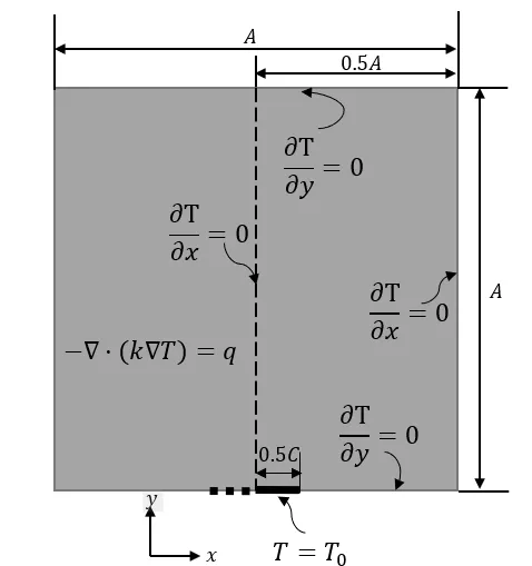
Figure 1: The volume-to-point problem.

Figure 2: Mesh resolution=200×200,500×500,700×700,800×800 from left to right. Volume fraction=0.2, σ=2.5×10-3, =500, C=0.05.

Figure 3: Mesh resolution = 700×700,800×800,950×950,1300×1300 from left to right. Volume fraction =0.2, σ=1.25×10-3, =500, C=0.05.

Figure 4: The objective versus the number of iterations. Volume fraction=0.2, Mesh resolution 500×500, σ=2.5×10-3, =500.

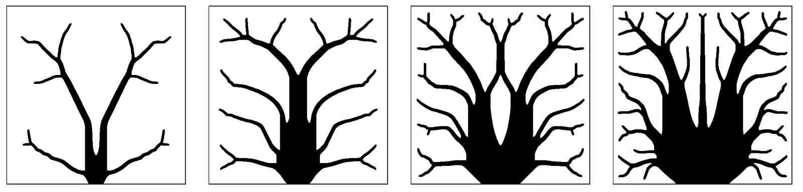
Figure 5: Volume fraction =0.1, 0.2, 0.3, 0.4 from left to right. Mesh resolution 500×500, σ=2.5×10-3, =500, C=0.05.

Figure 6: σ=1.5×10-4,2×10-3,2.5×10-3,3×10-3 from left to right. Volume fraction =0.2, mesh resolution 500×500, =500, C=0.05.

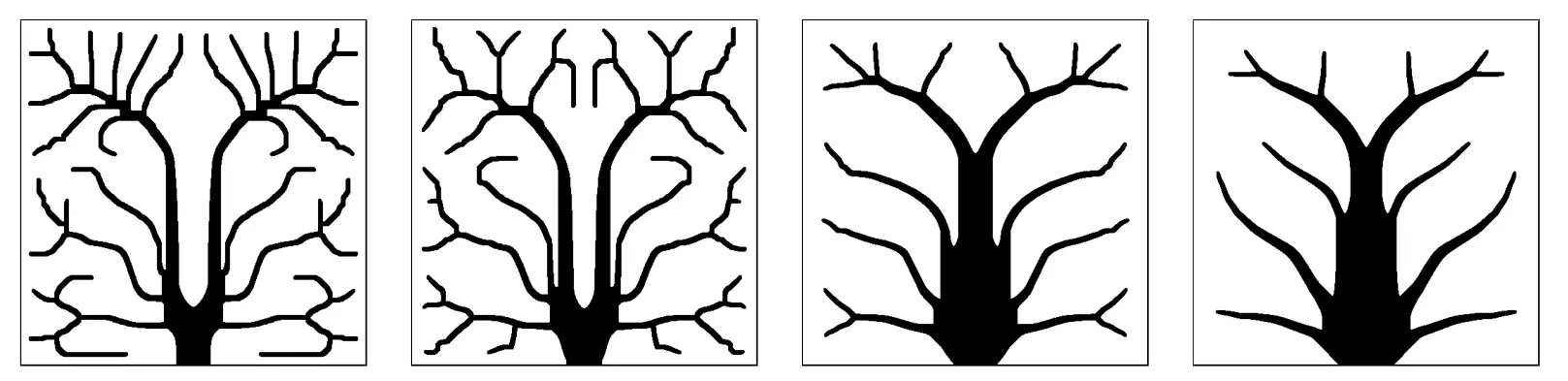
Figure 7: =50000,10000,500,100 from left to right. Volume fraction=0.2,mesh resolution 500×500,σ=1.25×10-3, C=0.05.

Fig. 5 shows the optimized distribution as the volume fraction (of the high conducting material) increases. The volume distribution tends to concentrate on the tree trunk, especially close to the isothermal boundary while the thickness of the smallest branches seems unchanged. When the volume fraction is the same, the optimized distribution depends on filter sizeσand conductivity ratio. In Fig. 6,whenσbecomes larger, we can see that the distribution contains less fine branches.This is because after convolution withGσthe fine branches will have lower conducting efficiency whenσis larger. Similarly when0becomes smaller, thin branches conduct heat less efficiently compared to whenis large. As shown in Fig. 7, asbecomes smaller, branches becomes thicker.

6.2 Volume-to-sides problem

Here we consider a square plate all of whose boundary is isothermal withT=T0as shown in Fig.8. Inside the plate,heat is generated uniformly. Due to symmetry,we only optimize over the upper left quadrant of the plate. On the vertical line and the horizonal line of symmetry (dashed lines in Fig. 8), we impose Neumann boundary conditions onT. We set volume fraction to be 0.5 andA=1.T0=0 and=50. The initial distribution is uniform and the convergence criterion is the same as that for the volume-to-point problem. The average number of iterations for the experiments presented here is 150.9. The results for different mesh resolution are shown in Fig.9.The distribution of the void region(white region)looks like a leaf in each quadrant of the plate. As the mesh is refined,the distribution stabilizes. Fig.10 shows that as the volume fraction of high conductive material increases,mainly those parts close to the vertical and horizontal symmetric lines of the plate get thickened, which effectively transfer heat generated in the center to the isothermal boundaries. The influence of the conductivity ratioand the filter sizeσto the optimized distribution can be seen in Fig. 11 and in Fig. 12 respectively. Similar to the volume-to-point problem,the results exhibit finer structures when the conductivity ratio becomes larger or the filter size becomes smaller.

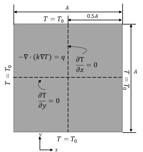
Figure 8: The volume-to-sides problem.

Figure 9: From left to right, mesh resolution is 500×500, 600×600, 1400×1400, 1600×1600.=100,σ=2.5×10-3. Volume-to-sides problem.

Figure 10: From left to right, volume fraction =0.1,0.2,0.3,0.4. σ=2.5×10-3, =100. Mesh resolution is 600×600.

Figure 12: From left to right, σ=2.5×10-3,5×10-3,1×10-2,2×10-2. Mesh resolution is 600×600.=500. Volume-to-sides problem.

7 Conclusions

By reformulating the heat transfer problem into a min-min problem,we developed a volume-preserving coordinate descent method, in which the characteristic function is updated by an iterative thresholding method. The method is simple to use and has the energy decaying property. The characteristic function gives a black-or-white design without need of post-processing. Numerical experiments are conducted to show the efficiency of the method. We also studied the effects of the conductivity ratio and filter size on the optimized distributions.

Appendix: Proof of Lemma 2.1

Proof. It is easy to see that R*=k∇T∈Sby(2.1b)and the definition ofS. We also have

Now we show thatR*minimizesoverS.∀R∈S,

Substituting R*withk∇Tfirst and then integrating by parts, we have

SinceT=T0on ΓD, R·n=R*·n=0 on ΓΓD,∇·R*=∇·R in Ω,

Therefore,

This completes the proof.

Acknowledgements

X.-P. Wang acknowledges support from National Natural Science Foundation of China (NSFC) grant (No. 12271461), the key project of NSFC (No. 12131010), the Hong Kong Research Grants Council GRF (GRF grants Nos. 16308421, 16305819,16303318) and the University Development Fund from The Chinese University of Hong Kong, Shenzhen (UDF01002028).