Nonisospectral Lotka–Volterra Systems as a Candidate Model for Food Chain

Xiao-Min Chen and Xing-Biao Hu

1 Institute of Applied Mathematics, Department of Mathematics, Faculty of Science, Beijing University of Technology, Beijing 100124, China

2 LSEC,ICMSEC,Academy of Mathematics and Systems Science, Chinese Academy of Sciences, Beijing 100190, China

3 School of Mathematical Sciences, University of Chinese Academy of Sciences, Beijing 100049, China

Abstract. In this paper, we derive a generalized nonisospectral semi-infinite Lotka–Volterra equation, which possesses a determinant solution. We also give its a Lax pair expressed in terms of symmetric orthogonal polynomials. In addition, if the simplified case of the moment evolution relation is considered,that is, without the convolution term, we also give a generalized nonisospectral finite Lotka–Volterra equation with an explicit determinant solution. Finally,an application of the generalized nonisospectral continuous-time Lotka–Volterra equation in the food chain is investigated by numerical simulation. Our approach is mainly based on Hirota’s bilinear method and determinant techniques.

Key words: Nonisospectral Lotka–Volterra, symmetric orthogonal polynomials, food chains, determinant techniques, Hirota’s bilinear method.

1 Introduction

It is known that Lotka–Volterra equation is an important biological model. Food chains withnmembers modelled by Lotka–Volterra equation are as follows [25]

with allrj,aij≥0, where the first population is the prey for the second, which is the prey for the third,and so on up to then-th,which is at the top of the food pyramid.Thexidenotes the density,riis intrinsic growth (or decay) rate, andaijdescribes the effect of thej-th upon thei-th population.ajj＞0 means speciesj’s population has a negative effect on itself, which attempt to prevent populations from growing indefinitely.

It is noted that in most literatures, the coefficientsaijof (1.1) are usually regarded as constants (see [13]), namely the system (1.1) is often considered as an autonomous system. This assumption of a constant environment is reasonable in some cases. Nevertheless, since biological and environmental parameters are naturally affected by time fluctuations in reality, a more realistic model would allow these parameters to change over time. Thus the studies on the non-autonomous Lotka–Volterra equation appear naturally. For instance, in [37], Teng and Yu considered a two-dimensional non-autonomous prey-predator Lotka–Volterra system,which corresponds to the casen=2 of (1.1) with the coefficientsriandaij(i,j=1,2)being continuous and bounded functions oftdefined on [0,∞). The extinction of the general non-autonomous predator-prey Lotka–Volterra system under some very weak assumptions is studied there. Besides, Meng and Chen in [31] studied a nonautonomous Lotka–Volterra almost periodic predator-prey dispersal system with discrete and continuous time delaying, which consists of n-patches. This system is uniformly persistent and globally asymptotically stable under some appropriate conditions, and owns a unique globally asymptotical stable strictly positive almost periodic solution. More relevant and rather incomplete examples modeled by the non-autonomous Lotka–Volterra system please consult [1,12,20–22,28,38].

In this paper, we study the Lotka–Volterra model from the view of integrable system. Apart from an important biological model, the Lotka–Volterra equation is also a classical integrable system. We obtain a nonisospectral Lotka–Volterra equation, which can be regarded as a non-autonomous food chain model withnspecies.Some qualitative analyses about the impacts of the corresponding coefficients have been done with the help of numerical simulations.

It is known that the Lotka–Volterra system has an intimate connection with the symmetric orthogonal polynomials. The semi-infinite Lotka–Volterra system(or the Kac-van Moerbeke lattice or the Langmuir lattice) [4,26,30,39]

can be regarded as a compatibility condition of Lax pair expressed in terms of the symmetric orthogonal polynomials (see [33]). To relate orthogonal polynomials to continuous-time integrable systems, the key idea is to introduce a one-parameter deformation of the measure, such that the measure and consequently corresponding orthogonal polynomials are also time-dependent [19,27,32,33].

Concretely speaking, a set of monic symmetric orthogonal polynomialsqn(x) is defined on a symmetric interval [-a,a] (acould be infinite) with an even weight function, that is,w(-x)=w(x) (see [18,33,35,36]). More precisely,qn(x) satisfy

wherehnare the normalization constants andδmnare the Kronecker delta. It is known that the monic symmetric orthogonal polynomialsqnsatisfy a three-term recurrence relationship

withq0(x)=1 andq1(x)=x. Clearly, these polynomials have the parity property

To make the symmetric orthogonal polynomialsqn(x) connected to the semiinfinite Lotka–Volterra system(1.2),assume thatqn(x)depend on an additional(socalled “time”)parametert(see[19]). This means that the recurrence coefficientsunbecome a function of the parametert,and the corresponding even weight function is also time-dependent,i.e.,w(x,t). Then the above three-term recurrence relationship becomes

with initial conditionsq0(x,t)=1 andq1(x,t)=x. Now assume that the relation [33]

holds for alln=1,2,···,withq-1(x,t)≡0, where the dot indicates the differentiation with respect totand this symbol is also valid in the sequel. Compatibility condition of (1.4) and (1.5) then yields the semi-infinite Lotka–Volterra system (1.2).

A tau-function solution of (1.2) is given as follows. Indeed, there is a one-to-one correspondence between the measure and the coefficientundefined in the above three-term recurrence relationship(1.4)ofqn. This is closely related to the classical moment problem. Let the moments corresponding to the even weight functionw(x,t)be denoted by

Apparently, all odd moments vanish,s2i+1(t)≡0. Denotecj(t)=s2j(t) for convenience, and assume that

withc0=φ(t),whereφ(t)is an arbitrary function. Furthermore,define two sequences of determinants

Then the determinant representations for the polynomialsqn(x) can be constructed below by using the orthogonality [19,34],

It is known that the coefficientun(t)of the recurrence relation(1.4)has the explicit determinantal expressions of the forms

which gives a solution of the semi-infinite Lotka–Volterra system (1.2). The linear differential equation (1.6) is a key equation which characterizes the tau-functionHmnof the semi-infinite Lotka–Volterra system (1.2). It is easy to check that (1.5)is automatically valid with the help of the determinant representations ofqngiven in (1.8) and the evolution relation (1.6) of the moments.

Another alternative approach to verify the above tau-function solution (1.9) is from the standpoint of Hirota’s bilinear method [24]. Regard the expressions in(1.9)as dependent variable transformations,then the corresponding Hirota’s bilinear forms of the semi-infinite Lotka–Volterra system (1.2) are as follows

with≡0 and1 form=0,1,2,···. The bilinear forms (1.10a)-(1.10b) are nothing but two Jacobi identities,or the so-called Sylvester determinant identities[7]by applying the linear differential equation (1.6).

Interesting work on the time-continuous Lotka–Volterra equation and symmetric orthogonal polynomials has been studied and elucidated (see [2,3,5,33]). In paper[33],from orthonormal polynomials and a(non-matrix)Stieltjes function,Peherstorfer et al. proved that the equation of motion of the Volterra chain is equivalent to the Riccati equation of Stieltjes function. This means that the evolution of the corresponding moment with respect totinvolves convolution terms. Moreover,in[5],Berezansky and Shmoish using the inverse spectral method derived a nonisospectral generalization of the classical Lotka–Volterra system by introducing a more general one-parametric family of the deformations of the even measures. Here nonisospectral integrable system means an integrable system possessing a nonisospectral Lax pair [8,10,14,23,29,40]. More relevant works can consult [9,15–17].

Motivated by the works in [5] and [33], in this paper, we obtain a generalized nonisospectral semi-infinite Lotka–Volterra equation

withu0(t)≡0,n=1,2,3,···, equipped with its corresponding Lax pair expressed in terms of the symmetric orthogonal polynomials. Our approach is from the perspective of Hirota’s bilinear method and determinant techniques. It is assumed that the form of the explicit solution remains the same as that of the classical Lotka–Volterra equation. We firstly alter the evolution relation with respect to time t for the moments of Hankel determinant, for instance, introducing an additional convolution term (see (3.1)). Then with the help of determinant identities, a nonisospectral Lotka–Volterral equation is derived. As mentioned above, the evolution relation of the moments plays a key role, such new evolution relation then determines a corresponding Lax pair in terms of symmetric orthogonal polynomials by applying the determinant representations (1.8). To the best of our knowledge, this generalized nonisospectral semi-infinite Lotka–Volterra equation with time evolution of the moments given by (3.1) is novel. Besides, a nonisospectral finite Lotka-Voltrerra equation(5.3a)with determinant solution is given as well in this paper if the convolution term is not considered in the evolution relation of moment. This nonisospectral finite Lotka–Voltrerra equation is a generalization of the finite Lotka–Voltrerra equation discussed in [19].

At the end of this paper, as an application, we regard the nonisospectral Lotka–Volterra equation proposed in the paper as a non-autonomous food chain model withnspecies. Notice that recently Erica Chauvet et al. in [11] considered an autonomous Lotka–Volterra three-species food chain, where they use numerical methods to qualitatively discuss the behavior of species. To compare with their results,we particularly discuss the three-species food chains case and use the numerical method of Runge Kutta to simulate the behaviors of each species. Numerical simulations show that the populations of each species at the maxima vary along time t and the moment that the maxima appear is also affected.

This paper is organized as follows. In Section 2,we give some important determinant identities, which are of great help in obtaining our main results. A generalized nonisospectral semi-infinite Lotka–Volterra equation and its explicit determinant solutions are presented in Section 3. Section 4 then follows to give a corresponding Lax pair expressed in terms of the symmetric orthogonal polynomials. In Section 5, we derive a nonisospectral finite Lotka–Volterra equation with the help of Hirota’s bilinear method and determinant techniques. Section 6 is committed to discussing an application of the generalized nonisospectral continuous-time Lotka–Volterra equation to food chain and some numerical simulations are demonstrated there. Section 7 is devoted to discussions.

2 Determinant formulae

Noting that the explicit formula for the solution of the Lotka–Volterra equation can be expressed in terms of the Hankel determinant, it is necessary to look for some underlying properties behind it. As we mentioned in the introduction, determinant technique has made a significant contribution to achieving our main results. In this section, we shall present some useful determinant identities independently.

For any determinantD, the well known Jacobi determinant identity [7] reads

Another important identity is the Schwein identity [7]. A Schwein identity of sizen+1 can be expressed as follows

where the elements of each matrix can be any numbers. In fact, it is easy to check that this Schwein identity follows immediately from applying the Jacobi identity(2.1) to

withi1=1,i2=n+1,j1=nandj2=n+1 respectively.

Now, let us introduce two new sequences of determinants below

Applying the Jacobi determinant identity (2.1) and Schwein identity (2.2), we have the following identities.

Lemma 2.1.Foranyintegern≥0,therehold

Proof. The proof for then=0,1 case is obvious by noting the convention≡0,Hm0≡1, Δm0≡0, Δm1≡1,Gm0≡0,Gm1≡cm+1, Γm1≡0, and Γm2≡(cm+1x2-cm+2) form=0,1,···.

Now we consider the case ofn≥2. The first two identities (2.4a) and (2.4b)can be proved by using the Jacobi identity (2.1). Applying (2.1) toD=and noticing that

identity (2.4a) is immediately obtained. In the same way, identity (2.4b) is the direct result of using Jacobi identity (2.1) to

with

Identity (2.4c) is simply applying Schwein identity (2.2) towithbj=x2jand=cn+jas well asai,j=ci+j, wherei=0,1,···,n-1 andj=0,1,···,n. Obviously, the identity (2.4d) which is similar to the formula (2.4c) can be obtained. Hence, we complete the proof of Lemma 2.1.

Corollary 2.1.Foranyintegern≥0,therehold

Proof. Noticing the determinant representations in (1.8) of the symmetric orthogonal polynomialsqn, it is easy to check that formulae (2.5a) and (2.5b) are the equivalent transformations of (2.4c) and (2.4d) respectively.

Besides, from the identities (2.4a) and (2.4b), we have

which leads to (2.5c) and (2.5d) immediately.

Furthermore, note that

then formulae (2.5e) and (2.5f) can be derived from (2.5c) and (2.5d), respectively.We complete the proof.

3 A generalized nonisospectral semi-infinite Lotka–Volterra equation

In this section, we will derive a generalized Lotka–Volterra system. It is noted that the Lotka–Volterra system(1.2)can be bilinearized into(1.10a)and(1.10b)through(1.9). Thus, in order to extend the system (1.2), it is natural to first generalize(1.10a) and (1.10b). To this aim, we have the following results.

Lemma 3.1.Assumethatthemoments{cj}satisfy

withc0=φ(t),wherea(t),b(t)andψ(t)aswellasφ(t)arearbitraryrealfunctions.Then,thedeterminantsHmnandGmndefinedin(1.7)and(2.3)withm=0,1satisfy thefollowingclosedbilinearforms

To prove this lemma, we first need the following lemma, which is related to the derivatives ofandH1n, respectively. Detailed proof can be found in Appendix A.

Lemma 3.2.

Now, we start to prove Lemma 3.1.

ProofofLemma3.1. Firstly, the last two equations in Lemma 3.1 are only two determinant identities (2.4a) and (2.4b), which we have shown in Lemma 2.1, respectively.

Then, by virtue of (3.3a) and (3.3b) and the identity (2.4a) we have

which gives (3.2a).

Similarly, by means of (2.4b), the following result holds true

which gives (3.2b). Thus, the proof of Lemma 3.1 is completed.

Now, by use of the bilinear forms exhibited in Lemma 3.1, we can extend the Lotka–Volterra system (1.2) to a generalized nonisospectral Lotka–Volterra system in the following theorem.

Theorem 3.1.Let

withu0(t)≡0,whereHmnwithm=1,2definedin(1.7),andtheevolutionofthe momentscjwithrespecttotimetsatisfiestherecurrencerelation(3.1).Thenun(n∈Z+)admitthefollowinggeneralizednonisospectralsemi-infiniteLotka–Volterra equation

Remark 3.1.Assume thata(t)≡2,b(t)≡1 andψ(t)≡0,then the reduced equation from (3.4)

can be transformed to the nonisospectral equation proposed by Berezansky and Shmoish in [5]:

after the change of variablesun=.

ProofofTheorem3.1. Without confusion,we abbreviate the functionsa(t),b(t)andψ(t) toa,bandψrespectively for convenience in the following proof. Bearing in mind (3.2a), identity (2.4a) as well as the results in Lemma 3.2, we getcan be expressed as

Then noticing the following useful formulas

and with the help of identity (2.5d), we obtain

Similarly, applying (3.2b) and the identity (2.5c), we have

Combining Eqs. (3.6) and (3.7) can lead to a conclusion that

thus (3.4) is valid and the proof of Theorem 3.1 is completed.

4 Lax pair in terms of symmetric orthogonal polynomials

As mentioned in introduction, the classical Lotka–Volterra equation can be derived as a compatibility condition of Lax pair expressed in terms of the symmetric orthogonal polynomials. For the generalized nonisospectral semi-infinite Lotka–Volterra equation (3.4) proposed in this paper, correspondingly, we can also construct a Lax pair from the perspective of the symmetric orthogonal polynomials. It is worth noting that, in this case the spectrum parameterxis dependent of timet.

For self-containedness, we recall the definition of the associated polynomials{Qn(x,t)}of the symmetric orthogonal polynomials{qn(x,t)}[6,p.77]. Let{qn(x,t)}be the symmetric orthogonal polynomials with the determinant expressions given in(1.8) andLdenote a linear function ofz, satisfying

Then,Qn(x,t) is defined by

whereLacts onz, andxandtare parameters. It is easy to see thatQn(x,t) is a polynomial of degree at mostninx, thatQ0(x)=0 and that, forn=1,2,3,···,

It is easy to check that the associated polynomials {Qn} satisfy the three-term recurrence relationship [6,33]

whereun+1(t)is the recurrence coefficient of(1.4)possessing the explicit expressions in(1.9). Actually,forn=2k,(4.2)is the consequence of applying the Jacobi identity(2.1) toD=2k+1withi1=k+1,i2=k+2 andj1=1,j2=k+2. And forn=2k+1,(4.2)is nothing but employing Schwein identity(2.2)toxQ2k+1withandai,j=ci+j+1fori=0,1,2,···,kandj=0,1,2,···,k+1.

With the help of the associated polynomials and the moment evolution relation given in (3.1), the following theorem of the characterization of the semi-infinite generalized nonisospectral Lotka–Volterra system (3.4) can be given.

Theorem 4.1.Letqn(x,t)bethesymmetricorthogonalpolynomialssatisfyingrecurrencerelationship(1.4),andassumethatthespectrumxisafunctionoftsatisfying

Thentherecurrencecoefficientun(t)ofqn(x,t)satisfiesthesemi-infinitegeneralized nonisospectralLotka–Volterrasystem(3.4)ifandonlyif

Remark 4.1.We can see from (4.3) that ifa(t)≠0, the spectrumxis dependent ontinstead of a constant, in other words, system (3.4) possesses a nonisospectral Lax pair fora(t)≠0.

Before proving Theorem 4.1, we need the following lemma first, which lists the results of direct calculations on the determinantsandby means of the evolution relations (3.1) and (4.3) of the momentscn(t) and the spectrumx(t)respectively. Its detailed proof is placed in Appendix B.

Lemma 4.1.Assumethemomentevolutionrelationsatisfies(3.1)andthespectrum xsatisfies(4.3),thentherehold

Now we are ready to give the proof of Theorem 4.1.

ProofofTheorem4.1. Similar to the proof of Theorem 3.1, without confusion, we abbreviate the functionsa(t),b(t)andψ(t)toa,bandψrespectively for convenience in the following proof.

The sufficient condition of Theorem 4.1 can be verified by the following three steps forn=2kandn=2k-1 respectively, wherek=1,2,3,···, and we omit the details.

Step 1. Differentiate the recurrence relationship (1.4) with respect totand then substitute the relations (4.3), (4.4a) and (4.4b) into it.

Step 2. Get rid of all the terms withQnby the recurrence relationship(4.2)and then replace all the terms with spectrum parameterxby a linear combination ofqnvia (1.4) to makexdisappeared. For instance,x2q2ncan be replaced by

Step 3. Use the fact that the symmetric orthogonal polynomials {qn(x,t)} are linearly independent polynomials to obtain the generalized nonisospectral semiinfinite Lotka–Volterra equation (3.4) forn=2kandn=2k-1 respectively.

Now, we turn to prove the necessary condition of Theorem 4.1. To begin with,from Theorem 3.1 we know that if the recurrence coefficientun(t) of (1.4) satisfies(3.4), thenun(t)possesses explicit expressions given in(1.9)with the moments evolution relation(3.1). Then with the help of(4.3),Lemma 4.1 and some determinant identities, we will show that formulas (4.4a) and (4.4b) can be verified easily by some direct calculations according to the determinant representations ofqngiven in(1.8).

More precisely,taking into account formulas(1.8),(3.3a)and(4.5a),and in view of identities (2.4c) and (2.5a), it is easy to obtain that

Then, employing identities (2.5c) and (2.5e) as well as the useful formula (3.5a), it yields

which coincides with (4.4a) and the validity of (4.4a) is hence verified.

Similarly, with the help of (1.8), (3.3b), (4.3) and (4.5b) as well as identities(2.4d),(2.5b)and(2.5f),it is not difficult to confirm(4.4b). Therefore,we complete the proof of the necessary condition of Theorem 4.1,and Theorem 4.1 is verified.

5 Nonisospectral finite Lotka–Volterra equation

In [19], Moody T. Chu mentioned a continuous-time finite Lotka–Volterra equation as follows:

which is Hamiltonian and also integrable. The dynamical system (5.1) enjoys a determinant solution

with

and the moments satisfy

whereφ(t) is an arbitrary function. This determinant solution can be utilized to effectuate numerical computation. A time integrable discretization of(5.1)has been implemented as an alternative means for the SVD computation [19], and the corresponding determinant solution can be applied to compute singular values of given rectangular matrices [39].

Since we have already obtained a continuous-time semi-infinite nonisospectral Lotka–Volterra equation from the standpoint of Hirota’s bilinear method and determinant techniques, it is natural to ask whether we can apply this method to seek a nonisospectral Lotka–Volterra equation for the finite case? This section aims to give a positive answer for this question. In fact, if the convolution term in the moment evolution relation(3.1)is not considered,we can generalize the finite Lotka–Volterra equation (5.1) discussed by Moody T. Chu to a nonisospectral case. This result is listed in the following Theorem.

Theorem 5.1.Anonisospectralcontinuous-timefiniteLotka–Volterraequationcan beexpressedas

whichownsageneralsolutionexpressedintheformof(5.2)with

Theevolutionofthemomentscjwithrespecttotimetsatisfiestherecurrencerelation asfollows

wherea(t),b(t)andφ(t)areknownarbitraryrealfunctions.

Proof. The condition≡0 plays an important role in this theorem, which we will prove first that it is compatible with the evolution relation(5.4)of the moments.

In fact, this mainly owes to the observation that the current momentscj(t)can also be defined as follows,

with the functionsλi(t) anddi(t) satisfying

Then, we have

which is in accord with (5.4).

To show that this definition of the momentscjimplies0 form=0,1,2,···as well, we first introduce the matrixform=0,1,2,···as

Since the momentscjare a linear combination ofdk,k=1,2,···,N, the matrixcan be decomposed into a product of two matrices, namely,

Based on the above decomposition, we see that the rank of the matrixis not greater thanN. Thus the corresponding determinant is vanished, that is,0,which shows that the condition0 is compatible with the evolution relationship (5.4) of the moments.

The evolution relationship of the moments is a bond that links Theorem 3.1 and Theorem 5.1 together. The evolution relationship (5.4) of the moments in Theorem 5.1 can be regarded as a reduction of the one(3.1)in Theorem 3.1 without the convolution term, that is, the case whenψ(t)≡0 in the latter. Therefore, we can make use of the results of Theorem 3.1 to prove Theorem 5.1.

Indeed, from Theorem 3.1 we know that,unwith the determinant expressions(5.2) and corresponding evolution relation (5.4) of the moments satisfies Eq. (5.3a)forn=1,2,···,2N-2. Hence, to prove Theorem 5.1, it remains to prove that Eq. (5.3a) is also valid for the casen=2N-1.

By using the condition (5.3b), Eq. (5.3a) forn=2N-1 can be rewritten as

Substitute the expressions (5.2) ofu2N-1andu2N-2into the above equation, then the right-hand of (5.5) reads

and the left-hand of (5.5) yields

Now,with the help of the bilinear equation(3.2b)and noticingψ(t)≡0 and0,there holds

Therefore, the left-hand of (5.5) finally can be expressed as

which can be easily checked that it coincides with (5.6) by using the identity (2.5d)and the conditionu2N≡0. Thus, we confirm that Eq. (5.3a) is also valid for the casen=2N-1 and Theorem 5.1 is verified.

6 Applications to food chain

Lotka–Volterra equation is a well-known biological model, and in the literature,numerical simulations are usually employed to analyze the behavior of each species.In this section, we regard the Lotka–Volterra equation (3.4) as a food chain model with n species. Without loss of generality, we particularly discuss the three-species food chains case and use the numerical method of Runge Kutta to simulate the behaviors of each species, and compare them with the results discussed by Chauvet et al. in [11] respectively.

Notice that assumeu0(t)=un+1(t)≡0,then Eq.(3.4)can be rewritten as follows

System (6.1) describes the food chain withnmembers, whereuidenote the densities. The coefficientais usually taken to be negative due to the termau2j, which means the speciesj’s population has a negative effect on itself, and thus intraspecific competitions with equal carrying capacity of each species are involved in (6.1).Instead of constantsaijin the Lotka–Volterra equation (1.1), here, the interaction between each predator and prey varies with respect tot. If takinga,b-2c0ψ(t)＜0,it means the first population is the prey for the second, which is the prey for the third,and so on up to then-th,which is at the top of the food pyramid. However,ifa≡0 andb-2c0ψ(t)＞0, it is easy to understand that (6.1) describes predator-prey interactions ofnspecies with each species preying on the next. Since this case is simpler and similar to the former case,we omit the details in this case in the sequel.Apparently, to investigate the influences on each species by variational interaction between each predator and prey, without loss of generality, we can choose the coefficientsa,bandc0as constants for simplicity, and only considerψ(t) as a function oftin (6.1).

Now without loss of generality, we take the three-species food chains withn=3 in (6.1) as an example, and use Runge Kutta method to simulate the behaviors of each biological species. Note that when it comes to describing the rate of change of population density, the intrinsic growth (or decay) rates of each species are usually taken into account. Thus to explore the effects of parametersa,band functionψ(t)on the food chains,we modify our initial model to make it more realistic and finally consider the following three-species food chains model:

withrj＞0,j=1,2,3,a≤0 andb-2c0ψ(t)＜0. Here the lowest-level preyis preyed upon by a mid-level species, which, in turn, is preyed upon by a top level predator. Examples of such three-species ecosystems include: mouse-snake-owl,vegetation-hare-lynx, and worm-robin-falcon.

The influence ofψ(t). The existence of functionψ(t) indicates that the intensity of each interaction between prey and predator of these three species is not only proportional to the populations of both species, but also varies with respect to timet.

To investigate the influences of the functionψ(t) on the behaviors of species clearly, we take the following nonlogistic three-species food chain model, discussed by Chauvet et al. in [11] as a reference model.

withrj＞0,a≤0 andb-2c0ψ＜0.

Note that the model (6.4) withψ(t)≡0 apparently will boil down to the model(6.3) with=x,=y,=zandr1=,r2=,r3=, 2a+b=-, 3a+b=-,b=-anda+b=-. Hence,to demonstrate the influences ofψ(t)on the behaviors of species, for convenience, now we only need to observe the behaviors modeled by(6.4) withψ(t)≡0 andψ(t)≠0 respectively. For the caseψ(t)≡0 in the model(6.4), which corresponds to the model(6.3), we display the three kinds of behaviors with respect toas well asexhibited in [11] in Fig. 1(a),Fig.2(a)and Fig.3(a)respectively. While for the caseψ(t)≠0 in the model(6.4),we take,as examples and observe their corresponding behaviors in Figs.1-3 respectively. It is worth noting that Figs.1(a)-3(a)correspond to Fig. 8 and Figs. 11 and 12 of [11] respectively, but the parameters chosen in Fig. 2(a) and Fig. 3(a) are different from those in Figs. 11 and 12 of [11]. The parameters chosen in the latter are inconsistent for the former,since the coefficients in model (6.4) are related to each other rather than totally independent in model(6.3). The concrete comparisons and analyses are listed below.

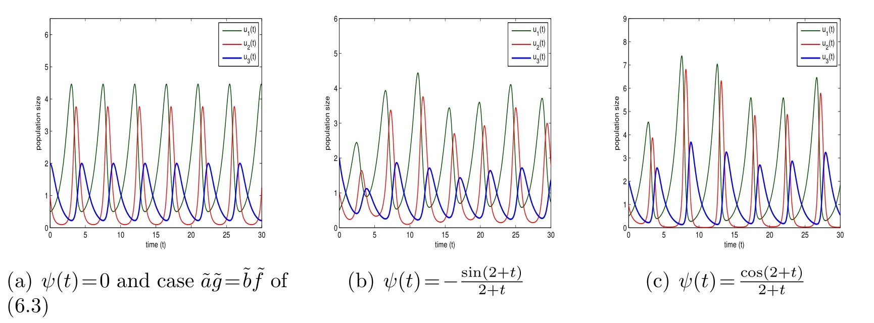
Figure 1: (6.4)with initial conditions((0),(0),(0))=(0.5,1,2)and r1=r2=r3=1,a=0,b=-1,c0=1.

Figure 2: (6.4) with initial conditions ((0),(0),(0))=(0.5,0.5,2) and r1=r2=r3=1, a=-0.1,b=-1, c0=1.

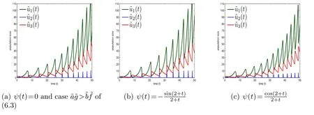
Figure 3: (6.4) with initial conditions ((0),(0),(0))=(0.5,1,2) and r1=0.5, r2=0.3, r3=0.25,a=-0.2, b=-0.5, c0=.

Therefore, the influences of functionψ(t) on the behaviors of species modeled by (6.4) are clear. Generally speaking, the populations of each species at the peaks vary along timetand the moment that the maxima appear is also affected. Now,we take the intraspecific competitions into accounts and turn to inspect the behavior of model (6.2).

The influences of the intraspecific competitions in (6.2).Model (6.2)of the three-species food chain witha＜0 describes more complicated and realistic biological behavior. On one hand, as discussed above, the interaction between each predator and prey varies with respect totinstead of a constant. On the other hand,the intraspecific competitions (theaterm), of all three species are considered.The carrying capacities of each species are -, which is the maximum number of individuals that can live stably in a population. We show below that the major impact of intraspecific competition is to reduce population growth rates as population density increases. Each species is likely to experience little or no intraspecific competition at low densities but intense intraspecific competition at high densities.

We first investigate the behavior of model(6.2)witha=-0.1 andand place the numerical simulation in Fig.4. Notice that all the parameters in Fig.4 are the same as those in Fig. 2(b) except for the extra influence of intraspecific competition. In contrast to Fig. 2(b), we can see from Fig. 4 that, the top speciesapproaches to extinction at a faster rate, with starting time of extinction beforet=40. The populations of the speciesandboth experience obvious fluctuations nearly beforet=60, as the densities are high and the intraspecific competitions are comparably intense, and then the speciesandboth tend to exhibit stable periodic behavior with very little intraspecific competitions.

Figure 4: (6.2)with the initial conditions((0),(0),(0))=(0.5,0.5,2)and r1=r2=r3=1,a=-0.1,b=-1, c0=φ(t)≡1 and ψ(t)=-

Figure 5: (6.2)with the initial conditions((0),(0),(0))=(0.5,1,2)and r1=0.5,r2=0.3,r3=0.25,a=-0.2, b=-0.5, c0=φ(t)≡ and ψ(t)= .

The influence of intraspecific competition is more conspicuous when it comes to the casein (6.3). Fig. 5 below exhibits the behavior of species depicted by model (6.2) with all the parameters being the same as those in Fig. 3(c) except for the extra influence of intraspecific competition. We can see from Fig. 5 that the behaviors of the speciesandare totally changed and the populations of them are no longer unbounded as shown in Fig. 3(c). Instead, the populations of all the three species tend to stable values quickly.

The above numerical simulations shown by Fig. 4 and Fig. 5 reveal that the intraspecific competition can indeed prevent populations from growing indefinitely.Fig. 5 in particular demonstrates the dramatic change in the populations of speciesandfrom unfettered growth in Fig. 3(c) to stable values with only slight fluctuations at the beginning. This is actually largely related to the value of parameter a, which is related to the carrying capacity of the species. The biggera(a＜0) is,the more fluctuations appear in the beginning. To show this, we choose a smaller value ofathan the one in Fig. 4 and a bigger value ofathan the one in Fig. 5 respectively. The numerical results are placed below.

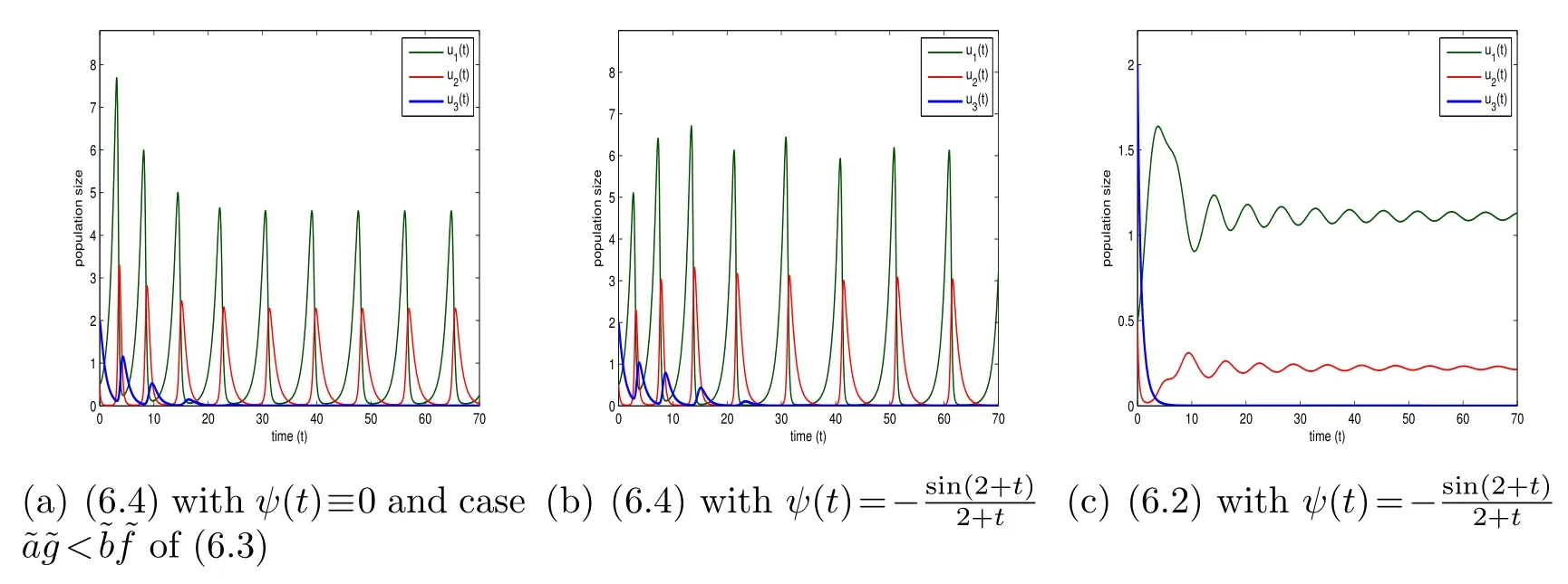
Figure 6: The initial conditions((0),(0),(0))=(0.5,0.5,2)and r1=r2=r3=1, a=-0.5, b=-1,c0=φ(t)≡1.

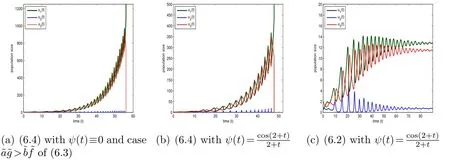
Figure 7: The initial conditions ((0),(0),(0))=(0.5,1,2) and r1=0.5, r2=0.3, r3=0.25,a=-0.01, b=-0.5, c0=φ(t)≡.

Fig.6 is to compare with Fig.4 with all the parameters the same as those in Fig.4 except for a smallera. Corresponding to Fig. 2(a), Fig. 2(b) and Fig. 4, Fig. 6(a),Fig. 6(b) and Fig.6(c) display the behavior of (6.3)in the case ofand(6.4)and (6.2) withrespectively. In contrast to Fig. 4 witha=-0.1 and obvious fluctuations at the beginning, Fig. 6(c) witha=-0.5 shows a sharp change of the behavior of all three species with very little fluctuations at the beginning and earlier stable periodic behavior. In the same manner, Fig. 7 is committed to comparing with Fig. 5, where Fig. 7(a), Fig. 7(b) and Fig. 7(c) correspond to Fig. 3(a), Fig. 3(c) and Fig. 5 respectively. The only difference between Fig. 7(c)and Fig. 5 isa=-0.01 in the former anda=-0.2 in the latter. We can see from Fig.7(c)that all the three species experience similar behavior to the one in Fig.3(a)and in Fig. 3(c) at the beginning and then tend to stable populations gradually.

7 Conclusions and discussion

In this paper, we have derived a generalized semi-infinite nonisospectral Lotka–Volterra equation with the solution of explicit determinantal expression. It possesses a Lax pair expressed in terms of the symmetric orthogonal polynomials. Besides,if the convolution term in the moment evolution relation (3.1) is not considered, a generalized nonisospectral finite Lotka–Volterra equation with its explicit determinant solution is also obtained. Our approach is primarily based on Hirota’s bilinear method and determinant techniques. At the end, we apply the generalized nonisospectral Lotka–Volterra equation to food chain withnmembers and investigate the impacts of the corresponding parameters by numerical simulations. For such a food chain, the intraspecific competition of each species is considered and the interaction between each prey and predator varies along with timetinstead of a constant assumed in most models.

Actually, since we also give a nonisospectral Lotka–Volterra equation in finite case(5.3a)-(5.3b)with an explicit solution(5.2),we try to apply this explicit solution to give a quantitative analysis of the behavior of biologic species.

Specifically,for the odd number of species,without loss of generality we take the three-species food chains as an example as well,which corresponds to the caseN=2 of Theorem 5.1. In order to get the similar form to model (6.2), we letu1=e-r1t,u2=andu3=er3twithrj＞0 (j=1,2,3) and substitute them into (5.3a),then there holds

with the following exact solutions by means of the formulas (5.2)

Here

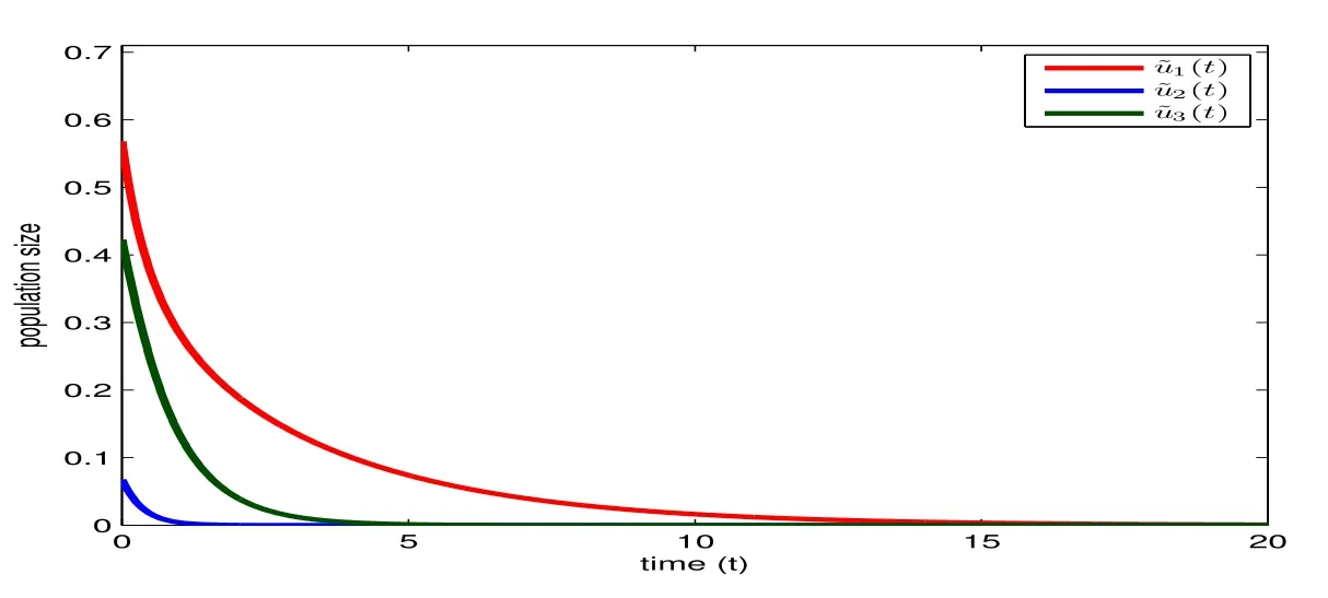
Figure 8: The exact solution of (7.1) with r1=0.3, r2=r3=0.5, a(t)≡b(t)=-e2r1(t+1), c0=e-4r1t+.

and according to the proof of Theorem 5.1, we can takec0(t) as

with

respectively. Now we consider an example of model (7.1) in detail. Taker1=0.3 andr2=r3=0.5 witha(t)≡b(t)=-e2r1(t+1), thus it is easy to obtain that

Moreover, for even-numbered species, we do not give an exact solution for model (5.3a). However, notice that if leta(t)≡0 then there hold(t)+(t)+···+(t)≡0 immediately in Theorem 5.1. It means that we can use the conserved quantityu1(t)+u2(t)+···+u2N-1(t)≡Cto obtain a model for even-numbered species, which possesses the exact solution as well. To show this clearly, without loss of generality we takea(t)≡0 andN=3 in Theorem 5.1 as an example,then it is easy to check thatby using of boundary conditions (5.3b). Assumeu1(t)+u2(t)+u3(t)+u4(t)+u5(t)≡Cand substituteu1(t)≡C-u2(t)-u3(t)-u4(t)-u5(t) into (5.3a), we obtain

In order to make model(7.4)more realistic to depict predator-prey relations between an even-numbered species, we takeuj=erj-1twithrj-1＞0 forj=2,3,4,5, and substitute them into (7.4), then there holds

with the exact solution

where

andc0(t) can be chosen as

with the constantsλifori=1,2,3. Now let us consider two concrete examples.

·Takeb(t)=sin(2+t)-2 andλ1=1,λ2=2,λ3=3 as well asr1=r2=r3=1,r4=2.

In this case, we have

immediately. Besides, with the help of Matlab, it is easy to check thatu1(t)+u2(t)+u3(t)+u4(t)+u5(t)≡6 and hence model (7.5) for the four species withC=6 can be described by its exact solutions via(7.6)and(7.7),which is shown in Fig. 9.

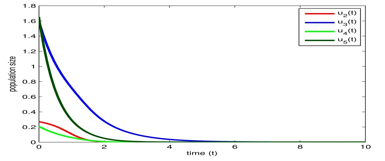
Figure 9: The exact solution of (7.5) with C=6 and r1=r2=r3=1, r4=2, and b(t)=sin(2+t)-2.

·Takeb(t)=andλ1=1,λ2=2,λ3=3 withr1=r2=1,r3=r4=0.3.Consequently, there is

withu1(t)+u2(t)+u3(t)+u4(t)+u5(t)≡6 as well. We plot the behavior of the four species modelled by (7.5) withC=6 through the exact solutions (7.6)with (7.7) in Fig. 10.

However, Figs. 8-10 clearly only describe the almost monotonous trend toward extinction of all biological species in the food chain,which seems strange to most food chains in reality. Therefore,with reference to those numerical simulations in Section 6, it is natural to ask whether the exact solution (5.2) of the finite nonisospectral Lotka–Volterra equation(5.3a)-(5.3b)can also be used to depict similar behavior of biologic species quantitatively? We shall consider these problems in the future.

Appendix

A Proof of Lemma 3.2

We prove Lemma 3.2 by the method of direct determinant calculations. For convenience, we first introduce some auxiliary notations as follows.

Denote

Then by virtue of the recurrence relations (3.1) of the momentscj, we have

Besides, by using the derivative relation (4.3) of the spectrumx, it yields

Using the above results (A.2), we have

Actually,expanding the determinantwith the(j+1)-th column,there holds

since

fori=0,1,···,n-1, thus (A.4a) is verified.

To check the formula (A.4b), we turn to first compute the determinant

which can be performed by implementing two types of the column operation. One,named as the left operation,is adding thep-th column multiplied by-cj+2-pto the(j+1)-th column forp=1,2,···,j, and the other one, named as the right operation,is adding the (j+2)-column multiplied by -c0to the (j+1)-th column.

Forj=0, we perform the right operation and get

And forj=1,2,···,n-1, after employing both the left operation and the right operation in the determinant |A0,···,Aj-1,Bj+1,Aj+1,···,An|, we find

Finally, forj=n, we only implement the left operation and obtain

Thus, there holdsand analogous to the proof of (A.4a), it is easy to verify that

which implies the validity of (A.4b).

Therefore, we justify (3.3a) of the derivative of. (3.3b) can also be proved following the similar process to (3.3a) and we omit its detailed proof. The proof of Lemma 3.2 is hence completed.

B Proof of Lemma 4.1

Based on the moment evolution relation (3.1), Lemma 4.1 can be proved by the method of direct determinant calculations. We still use the notations defined by(A.1a) and (A.1b) in Appendix A.

By applying (A.2) and (A.3), we have

Note that

To verify(B.1a),we expand the determinantwith the(j+1)-th column and obtain that(B.1a) is hence confirmed.

For the formula (B.1b), similar to the proof of (A.4b), we apply the two types of the column operation, namely the left operation and the right operation, to the determinant |A0,A1,···,Aj-1,Bj+1,Aj+1,···,An-1,X|. The detailed results are list below.

Forj=0, we act the right operation in |B1,A1,······,An-1,X| and obtain

and for the case whenj=1,2,···,n-2, performing both the left operation and the right operation lead to

In the end, forj=n-1, applying the left operation only, we have

Thus, there holds

To confirm (B.1b), it remains to calculate the last term of the above equation.

In fact, by expanding the determinantwith the (j+1)-th column, we get

Since (B.2) plays an important role in the proof ofsatisfying (4.5a), we elaborate on its detailed calculations. Notice that in casek=0, it yields

Fork=1,2,···,n-2, there holds

Finally, fork=n-1, it leads to

where we use the following identity

which is nothing but invoking (1.8) and applying Jacobi identity (2.1) to the determinantD=2n+2withi1=n+1,i2=n+2 andj1=n+1,j2=n+2.

Thus, with the help of (4.1a) and (B.2), we obtain

which implies that(B.1b)is valid and the first formula(4.5a)in Lemma 4.1 is hence confirmed.

Since by invoking (4.1b), formula (4.5b) ofcan be proved via analogous calculations to the proof of the formula (4.5a) ofwe omit the detail. This completes the proof of Lemma 4.1.

Acknowledgements

X.M.Chen was supported by R&D Program of Beijing Municipal Education Commission (Grant No. KM202310005012), National Natural Science Foundation of China (Grant Nos. 11901022 and 12171461), and Beijing Municipal Natural Science Foundation (Grant Nos. 1204027 and 1212007). X. B. Hu was supported in part by the National Natural Science Foundation of China (Grant Nos. 11931017 and 12071447).