蛋白质结构确定领域中的几种矩阵填充算法的对比评估*

李志诚 韦 仙 李晋婷

（1）太原师范学院物理系，晋中 030619；2）太原师范学院计算物理与应用物理研究所，晋中 030619；3）太原工业学院理学系，太原 030008）

Proteins are composed of ordered amino acid chains, which are vital macromolecules of cells in organisms. Determining the three‑dimensional structure of proteins is central to biophysics and bioinformatics because it is important to understand the physical, chemical and biological properties of proteins and to analyze possible interactions with other proteins[1]. X‑ray diffraction (XRD)crystallography was the main tool for obtaining protein information in the early period of protein structure determination[2]. However, the introduction of the nuclear magnetic resonance(NMR)technique is a breakthrough because NMR made it possible to obtain protein information in an aqueous environment much closer to the native state of a protein[3‑4]. The protein NMR method conventionally involves sample preparation, peak picking, spectral assignment,nuclear Overhauser effect spectroscopy (NOESY)[5‑6]assignment, structure calculation and refinement[7]as demonstrated in Figure 1. Because long distances(＞5 Å, 1 Å=10-10m) are difficult to be measured by NMR experiment[8], lacking sufficient distance information is the main challenge for this problem.To this end,the protein NMR methods rely profoundly on complex computational algorithms and techniques, e.g.distance geometry[9‑12],molecular dynamics[13‑15].

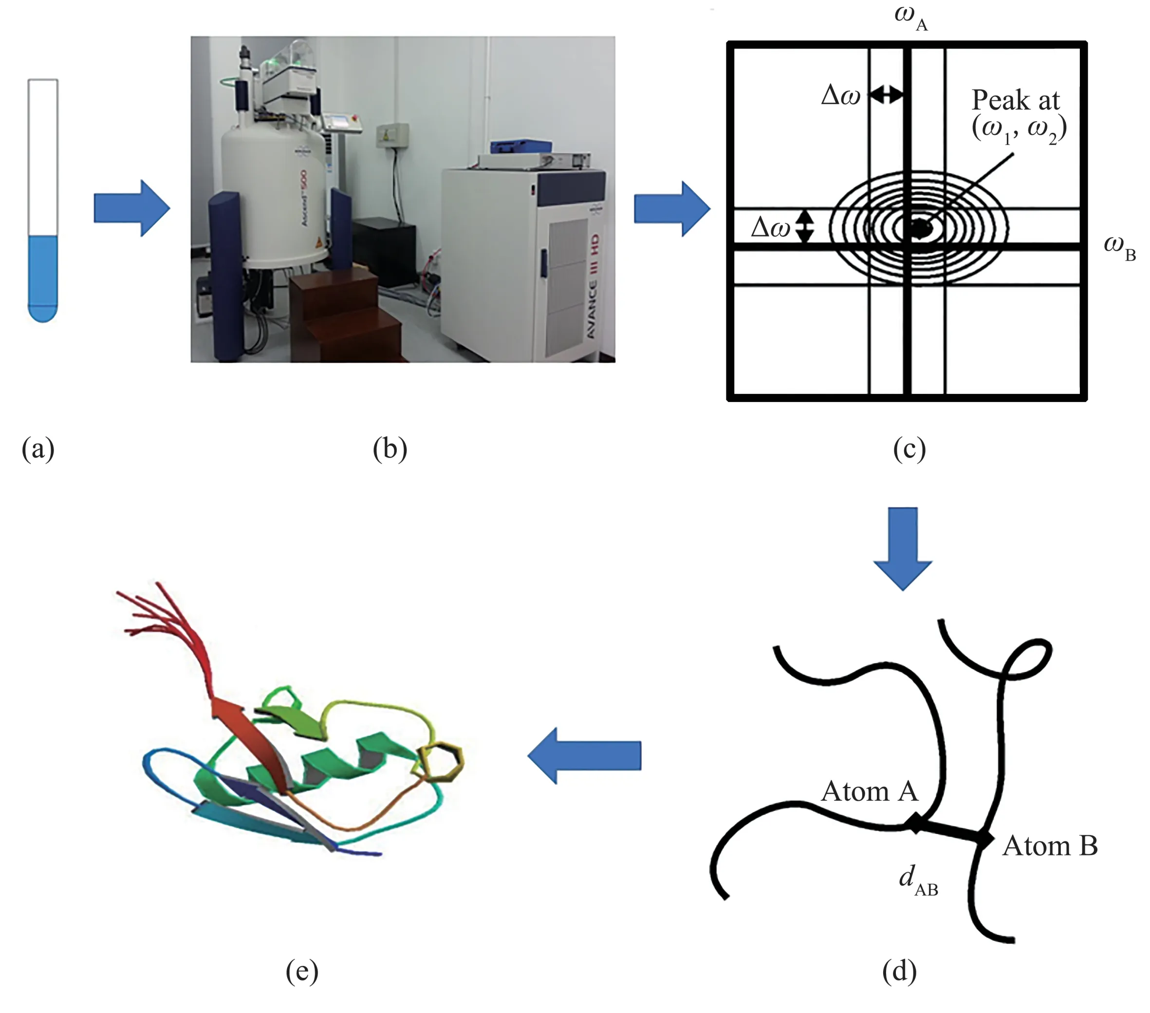
Fig.1 The procedure of protein NMR structure determination(a) Sample preparation: NMR experiments can directly measure protein samples in solution state; (b) NMR experiments: involving peak picking,spectral assignment, nuclear Overhauser effect spectroscopy (NOESY) assignment; (c) NMR spectroscopy: the sources of experimental data;(d)Distance constraints:obtaining a set of distance constraints from spectrums(the intensity of an NOE is the 6th power inversely proportional to the distance between two nuclei);(e)Structural calculation:the resulting geometric restraints are used as input for the structural calculation.

The proposed matrix completion (MC)theory[16‑17]provides a promising way to solve this problem. MC aims at recovering a low‑rank matrix from a partial sampling of its entries.In the early stage of MC development, one typical example is the famous Netflix problem, which aims to predict the user’s preferences for different types of movies based on a very sparse existing data set.In 2009,Candès and Recht[18]proposed that a matrix could be recovered with a very high probability if the number m of sampled entries obeys m≥Cn1.2rlogn, where C is a positive constant, n and r are dimension and rank of the matrix, respectively. Subsequently, Candès and Tao[19]improved this result to m≥Cnrlogn. Afterward Gross[20]generalized the standard MC problem by proposing a simpler and more general method. In the meantime, the MC problem with noise was also proposed. Candès and Plan[21]proposed that a matrix could be recovered accurately with Gaussian random noise and bounded noise if m obeys m≥Cnrlog6n.With the development of MC theory, it has received increasing interest and has been applied to various fields,such as protein structure calculation[22‑25],image processing[26‑27],traffic sensing[28].

In this paper, the protein NMR structure determination is addressed as an MC problem. In our previous work, the MC‑based accelerated proximal gradient (APG)[29]algorithm and scaled alternating steepest descent (ScaledASD)[26]algorithm have been investigated in recent years. In 2017, we applied the APG algorithm to protein structure calculation and demonstrated the effectiveness of the algorithm by analyzing the accuracy and error of the calculation results[22]. In 2019, a new algorithm, ScaledASD,originally applied in image processing, was tested for protein structure calculation, the results show the algorithm overcomes the shortcomings of insufficient NMR data to a certain extent[23].To further explore the effectiveness of MC in the field of protein structure estimation,6 MC algorithms were selected to be tested and compared their performance in this paper. The remainder of the paper is organized as follows:Section 1 gives a detailed description of our method including the problem model, MC and quality assessment.In Section 2,we evaluate the performance of 6 different MC algorithms under accurate sampling as well as noisy sampling, and make a detailed analysis. Finally, the conclusions and some perspectives are elaborated in Section 3.

1 Methods

1.1 Problem model

For a protein molecule, each atom can be considered as a three‑dimensional point in space. We assume the target protein has n atoms,then the protein structure consists of a set of points{x1,x2,…,xn},xi∈R3.The coordinate matrix is defined as X=[x1; x2; … ;xn] ∈Rn×3. Based on this, we can define a Euclidean distance matrix (EDM), whose elements stand for the distance between two atoms,such that

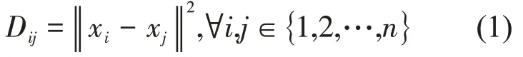
where‖ ‖x is the Euclidean distance norm of vector x.Obviously, we can transform a coordinate matrix X into a Euclidean distance matrix D according to Equation (1). Conversely, a Euclidean distance matrix D can also be converted back into a coordinate matrix X by a general approach[30]. In detail, we induce the Gram matrix G = XXT. Gram matrix G and distance matrix D have the following transformation relations:

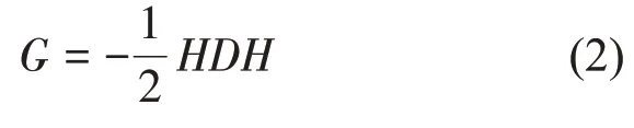
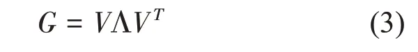
where V is an n×n square matrix, and Λ is a diagonal matrix in which the elements on the diagonal are the corresponding eigenvalues. Then the coordinate matrix corresponding to the protein structure is calculated as:

That is to say, a protein structure can be determined as long as the complete distance matrix is known.

Although we can gain some partial short distances from NMR experiments and some covalent bond lengths information[31], the distance data are still too sparse to determine a protein structure. To ameliorate this situation, MC algorithms are used to recover the incomplete initial distance matrix. Taking into account the condition of the uniform sampling distribution, we will sample the remaining distances randomly. Once the distance matrix is recovered, the protein structure is determined in light of the previous discussion. The proposed framework is shown in Figure 2.

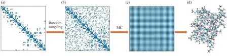
Fig.2 The schematic diagram of protein structure determination based on MC(a) The contour of the distance matrix containing only known short distances, including the atomic distances obtained from NMR experiments and covalent bond lengths; (b) The contour of the distance matrix after random sampling; (c) The contour of the complete distance matrix recovered by MC;(d)Transforming the complete distance matrix into a three‑dimensional protein structure.

1.2 Matrix completion （MC）

As explained previously, MC is the problem of recovering a low‑rank matrix from partial entries. A direct approach is to find a matrix D with the minimum rank that best approximates the underlying matrix D0:

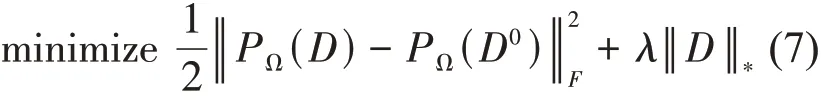
where Ω is a set of the indices for known elements,PΩdenotes the sampling operator restricted to the entries indexed by Ω, that is, D has the same elements as D0for the entries in Ω. Solving the problem (5) is challenging because rank minimization is non‑convex and generally NP‑hard[18]. A convex and tractable approach is proposed to replace the rank objective with the nuclear norm[32], then the problem (5) can be approximated by the following formulation:

where ‖ ‖D*denotes the nuclear norm of matrix D,namely, the sum of its singular values.To enhance the anti‑noise performance of the problem, an alternative and stable approach is used by relaxing the equality constraint:

where‖ ‖·Fdenotes the Frobenius norm of the matrix,λ is a parameter that controls the rank of matrix D. In this process, it is necessary to compute a singular value decomposition(SVD)[33]in each iteration.There have been many algorithms proposed for the problem(7), such as the accelerated proximal gradient (APG)algorithm[29], the hard thresholding algorithms[17]and the scaled gradients on Grassmann manifolds(ScGrassMC)method[34].

Taking into account the computational complexity of SVD, an alternative method based on matrix factorization was proposed. In detail, for an n‑dimensional distance matrix D,it can be written into a simple factorization form:D=XY where X∈Rn×rand Y∈Rr×n(r is the rank of the matrix). Then the problem is transformed into solving the minimization of the following function:

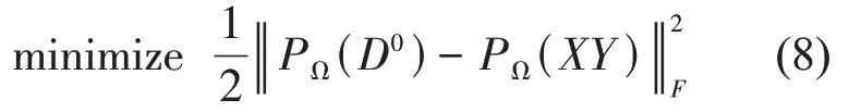
Solving the problem (8) generally uses an alternating minimization approach, which is widely used for optimization problems. The algorithms based on the matrix factorization model include low‑rank matrix fitting (LMaFit) algorithm[35], alternating steepest descent (ASD) algorithm and its scaled variant(ScaledASD)[26].

1.3 Quality assessment

In the field of structural biology, the accuracy of a molecular conformation is generally measured by the root‑mean‑square deviation (RMSD), which is a measure of the “average” deviation between the computed structure and the reference structure.Assume X denotes the computed configuration optimally aligned to the reference configuration X*by the alignment procedure[36],then the RMSD is defined by the following formula:

where n is the number of atoms, xidenotes the coordinate of the ith atom. A more accurate structure corresponds to a smaller RMSD value. Typically, the RMSD value less than 2 Å represents a high‑resolution model[37].

2 Results and discussion

In this paper, we studied the protein structure determination problem using 6 MC algorithms, listed in Table 1. Four proteins with different topological structures were selected as the target protein for testing in Table 2.For simplicity,we just took 1G6J as an example in this section. For the other proteins,similar results are obtained in Supplementary.All the tests in our work were carried out on a Windows 10 PC with a 3.1 GHz Intel Core i9‑9900 CPU and 32 GB of memory. In our test, the information of the initial distance matrix includes short distances (less than 5 Å) between hydrogen atoms and covalent bond lengths. To reach the sampling conditions of MC, the remaining distances need to be randomly sampled.For testing purposes, we firstly presume the sampling distances are accurate, and the case of the sampling distances with noise is discussed in 2.2.

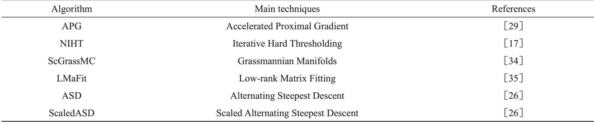
Table 1 List of MC algorithms evaluated in this paper

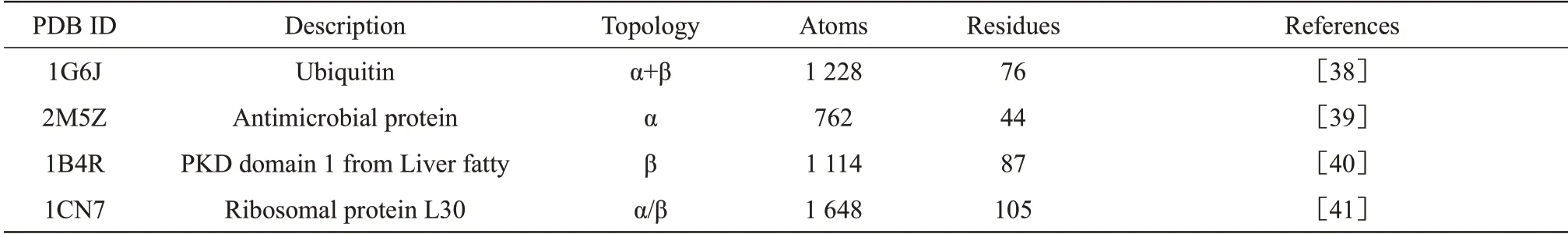
Table 2 The information of four test proteins

2.1 Results for 6 MC algorithms under accurate sampling

To evaluate the performance of the aforementioned algorithms, we calculate the RMSD related to all atoms between the reconstructed structure and the reference structure in the case of accurate sampling under the sampling ratios ranging from 1% to 10%. The corresponding Protein Data Bank (PDB)[42]model is selected as the reference structure. For all the aforementioned algorithms, the number of the maximum iteration and the relative residual tolerance is set to 500 and 10-5, respectively.For each algorithm and each sampling ratio, we calculated 100 times randomly and recorded the average value and standard deviation of the RMSD and the computational time. The standard deviation can reflect the stability of calculation results statistically, namely, a smaller standard deviation indicates a more stable calculation result. The results are shown in Figure 3.

Fig.3 The performance curve of 6 algorithms with different sampling ratios ranging from 1%to 10%for testing 1G6J(a)The average RMSD value,denoted by RMSD(ave);(b)The standard deviation of RMSD,denoted by RMSD(std);(c)The average computational time,denoted by Time(ave);(d)The standard deviation of computational time,denoted by Time(std).

Figure 3 shows the visual comparison of the aforementioned 6 algorithms applied to protein structure determination under precise sampling. For comparison purposes, we adjusted the scale range of the average value and the standard deviation to be consistent. Figure 3a shows the RMSDs (ave) for 6 algorithms. Naturally, with the increase of sampling ratio, the RMSDs (ave) become smaller, indicating that the calculational accuracy of algorithms becomes higher. Although the RMSDs (ave) are relatively larger with low sampling ratios, when the sampling ratio exceeds 3%,almost RMSDs(ave)are below 2 Å for all the algorithms (except the NIHT for 1B4R shown in Figure S1), that is to say, high accuracy can be obtained. Notably, when the sampling ratio exceeds 7%, the RMSD values are almost close to 0,indicating that the recovered structures are high‑resolution extremely.As can be seen in Figure 3b, the RMSD (std) tends to decrease as the sampling ratio increases. Especially under high sampling ratios(more than 7%), all the RMSDs (std) are almost close to 0, that is, the calculation of the algorithms turns to be more stable under high sampling ratios.According to Figure 3a, b, ScGrassMC is slightly more prominent than other algorithms, because its RMSDs(ave) and RMSDs (std) are relatively lower in most sampling ratios. Figure 3c shows the average computational time,by and large,the calculation costs less time with the increase of sampling ratio for all the algorithms. This seems to be natural because the scarcity of initial data can lead to more computations.NIHT and APG cost relatively more time, especially under low sampling ratios, while the computational times are significantly reduced under high sampling ratios. In Figure 3d, we can see that the Times (std)have lower values with high sampling ratios. On the whole,LMaFit and ScaledASD are more prominent in computational time because they cost less computational time and are more stable. Similar results with different sampling ratios for testing 1B4R, 2M5Z, 1CN7 are shown in Figure S1-S3,respectively.

2.2 Results for 6 MC algorithms under noisy sampling

In practical molecular conformation problems,the distance information tends to bring some noise, so it is instructive to consider the noise resistance ability of the algorithm in protein structure determination.To evaluate the anti‑noise performance of the aforementioned algorithms, different levels of noise are added to the sampling distances. In this paper, we have tested with a “normal” noise model akin to Reference [43], i.e., the noisy distances dˉijare given by:

where σ is a positive parameter, called noise factor,the value of zijaccords with standard normal distribution N(0, 1), dijis the accurate sampling distance. Obviously, the noise level can be controlled by the noise factor σ, the noise becomes larger as the value of σ increases.In this section,the sampling ratio is set to 10%, and each test is still calculated 100 times randomly.

We can see in Figure 4a, the RMSDs (ave)become larger and larger following the increasing noise factor. All the algorithms are still able to produce a fairly accurate structure (RMSD＜2 Å)when the noise factor is less than 15%. Meanwhile,within this noise range, the RMSDs (std) are also relatively stable according to Figure 4b. If the noise factor exceeds 15%, the RMSDs (std) become larger,that is, the stability of calculational accuracy is worse in high noise situations. Figure 4c shows the average computational time under different levels of noise. It is not immediately obvious that the computational time and noise have an explicit correlation. However,ScGrassMC and NIHT cost more computational time than other algorithms. Compared with Figure 3c, the computational time of the two algorithms is more sensitive to noise. We infer that the noisy distance data increases the number of iterations of calculation,which makes the computational time longer. Taking the ScGrassMC algorithm with a sampling ratio of 10% as an example, when there is no noise, the average number of iterations of calculation is 34,while when the noise factor reaches 10%, the average value of the number of iterations is 500, which is the maximum iteration set in our test.From Figure 4d,for most algorithms,Times (std) are small, indicating that the computational time is relatively stable. In comparison, the Times (std) of NIHT are slightly larger, and the Times (std) of ScGrassMC are larger only in high noise. Overall, in the case of noisy sampling distances, ASD and ScaledASD perform superior both in terms of computational accuracy and computational time. Similar results in the case of sampling distances corrupted different levels of noise for testing 2M52, 1B4R, 1CN7 are shown in Figure S4-S6 respectively.

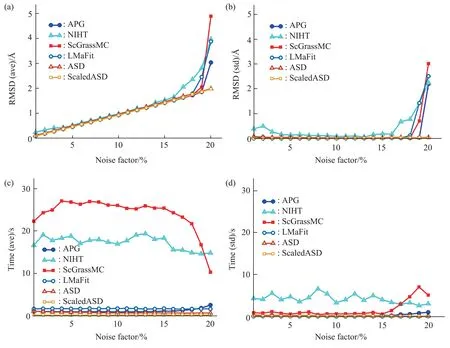
Fig.4 The performance curve of six algorithms in the case of sampling distances corrupted different levels of noise for testing 1G6J(a)The average RMSD value,denoted by RMSD(ave);(b)The standard deviation of RMSD,denoted by RMSD(std);(c)The average computational time,denoted by Time(ave);(d)The standard deviation of computational time,denoted by Time(std).

3 Conclusion and future work

In this paper, we have evaluated 6 MC algorithms applied to the protein structure determination problem. MC algorithms can effectively overcome the shortcomings of insufficient NMR experimental data. We took 4 proteins with different topological structures as examples to test the accuracy, computational time and noise resistance of these algorithms. Our test results show that the algorithms perform higher accuracy and shorter computational time with the increase of sampling ratio, and the stability of the algorithms is also higher.Especially, when the sampling ratio exceeds 3%,almost RMSDs are less than 2 Å, and when the sampling ratio exceeds 7%,the RMSDs are close to 0,which shows that all these algorithms can efficiently generate an accurate structure. A conclusion can be made that the algorithms perform remarkably well when there are enough exact distance data. By comparison, the ScGrassMC algorithm performs better in terms of computational accuracy, while LMaFit and ScaledASD are more advantageous in terms of computational time. Subsequently, we tested the noise resistance of the 6 algorithms by building the normal noise model. The computational accuracy decreases with the increase of noise, while when the noise factor is less than 15%, almost RMSDs are less than 2 Å, indicating all algorithms can produce relatively accurate structures in this situation. An interesting conclusion is that the NIHT and ScGrassMC algorithms cost significantly more computational time in the presence of noise,indicating that the computational times of both algorithms are sensitive to noise. ASD and ScaledASD have better noise resistance performance,both in terms of computational accuracy and computational time.The results of this paper give us a degree of confidence that the MC algorithms are promising in the field of protein structure determination. In the future, a further study on algorithmic mechanisms is our next work, which would help us to establish a greater degree of accuracy and efficiency in this field. We also believe that the results of this paper can potentially promote the development of more effective new MC algorithms in the future.

Supplementary PIBB_20210278_Doc_S1.pdf is available online(http://www.pibb.ac.cn or http://www.cnki.net).